Regularization of the AVO inverse problem by means of a ...

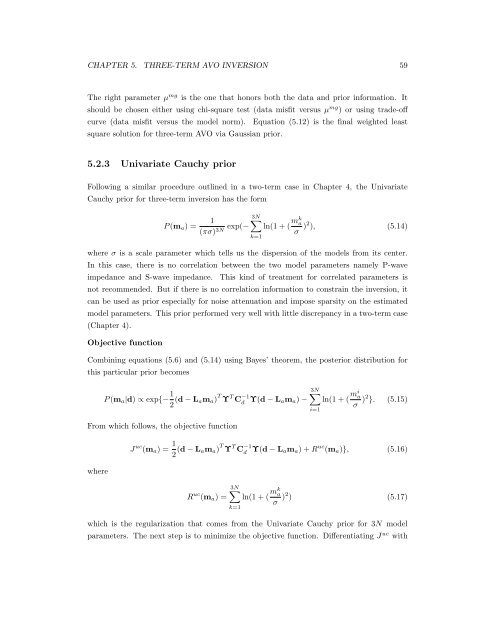
CHAPTER 5. THREE-TERM AVO INVERSION 59
The right parameter µ mg is the one that honors both the data and prior information. It
should be chosen either using chi-square test (data misfit versus µ mg ) or using trade-off
curve (data misfit versus the model norm). Equation (5.12) is the final weighted least
square solution for three-term AVO via Gaussian prior.
5.2.3 Univariate Cauchy prior
Following a similar procedure outlined in a two-term case in Chapter 4, the Univariate
Cauchy prior for three-term inversion has the form
P (ma) =
1
exp(−
(πσ) 3N
3N
k=1
ln(1 + ( mk a
σ )2 ), (5.14)
where σ is a scale parameter which tells us the dispersion of the models from its center.
In this case, there is no correlation between the two model parameters namely P-wave
impedance and S-wave impedance. This kind of treatment for correlated parameters is
not recommended. But if there is no correlation information to constrain the inversion, it
can be used as prior especially for noise attenuation and impose sparsity on the estimated
model parameters. This prior performed very well with little discrepancy in a two-term case
(Chapter 4).
Objective function
Combining equations (5.6) and (5.14) using Bayes’ theorem, the posterior distribution for
this particular prior becomes
P (ma|d) ∝ exp{− 1
2 (d − Lama) T Υ T C −1
d Υ(d − Lama)
3N
− ln(1 + (
i=1
mia σ )2 }. (5.15)
From which follows, the objective function
where
J uc (ma) = 1
2 (d − Lama) T Υ T C −1
d Υ(d − Lama) + R uc (ma)}, (5.16)
R uc (ma) =
3N
k=1
ln(1 + ( mk a
σ )2 ) (5.17)
which is the regularization that comes from the Univariate Cauchy prior for 3N model
parameters. The next step is to minimize the objective function. Differentiating J uc with