Regularization of the AVO inverse problem by means of a ...

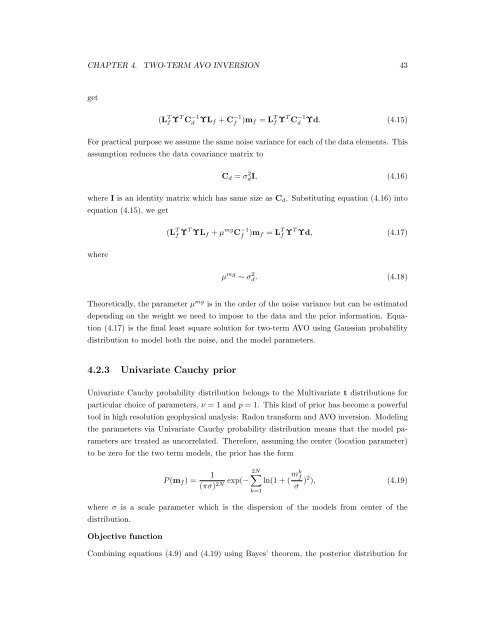
CHAPTER 4. TWO-TERM AVO INVERSION 43
get
(L T f Υ T C −1
d ΥLf + C −1
f )mf = L T f Υ T C −1
d
Υd. (4.15)
For practical purpose we assume the same noise variance for each of the data elements. This
assumption reduces the data covariance matrix to
Cd = σ 2 dI, (4.16)
where I is an identity matrix which has same size as Cd. Substituting equation (4.16) into
equation (4.15), we get
where
(L T f Υ T ΥLf + µ mg C −1
f )mf = L T f Υ T Υd, (4.17)
µ mg ∼ σ 2 d. (4.18)
Theoretically, the parameter µ mg is in the order of the noise variance but can be estimated
depending on the weight we need to impose to the data and the prior information. Equa-
tion (4.17) is the final least square solution for two-term AVO using Gaussian probability
distribution to model both the noise, and the model parameters.
4.2.3 Univariate Cauchy prior
Univariate Cauchy probability distribution belongs to the Multivariate t distributions for
particular choice of parameters, ν = 1 and p = 1. This kind of prior has become a powerful
tool in high resolution geophysical analysis: Radon transform and AVO inversion. Modeling
the parameters via Univariate Cauchy probability distribution means that the model pa-
rameters are treated as uncorrelated. Therefore, assuming the center (location parameter)
to be zero for the two term models, the prior has the form
P (mf ) =
1
exp(−
(πσ) 2N
2N
k=1
ln(1 + ( mk f
σ )2 ), (4.19)
where σ is a scale parameter which is the dispersion of the models from center of the
distribution.
Objective function
Combining equations (4.9) and (4.19) using Bayes’ theorem, the posterior distribution for