Introduction to regression

Chapter 3 Introduction to regression 115
Fitting a straight line — least-squares
regression
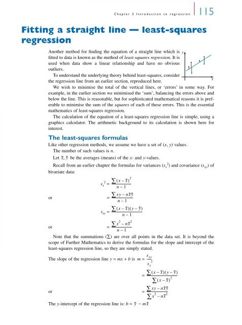
Another method for finding the equation of a straight line which is y
fitted to data is known as the method of least-squares regression. It is
used when data show a linear relationship and have no obvious
outliers.
To understand the underlying theory behind least-squares, consider
x
the regression line from an earlier section, reproduced here.
We wish to minimise the total of the vertical lines, or ‘errors’ in some way. For
example, in the earlier section we minimised the ‘sum’, balancing the errors above and
below the line. This is reasonable, but for sophisticated mathematical reasons it is preferable
to minimise the sum of the squares of each of these errors. This is the essential
mathematics of least-squares regression.
The calculation of the equation of a least-squares regression line is simple, using a
graphics calculator. The arithmetic background to its calculation is shown here for
interest.
The least-squares formulas
Like other regression methods, we assume we have a set of (x, y) values.
The number of such values is n.
Let x, y be the averages (means) of the x- and y-values.
2 Recall from an earlier chapter the formulas for variances (sx ) and covariance (sxy) of
bivariate data:
2
2 ( x – x)
sx = ------------------------ ∑
n – 1
or = ∑ xy–
nxy
------------------------n
– 1
( x – x)
( y– y)
sxy = ∑------------------------------------- n – 1
x
or =
Note that the summations (∑) are over all points in the data set. It is beyond the
scope of Further Mathematics to derive the formulas for the slope and intercept of the
least-squares regression line, so they are simply stated.
2
∑ nx 2
–
-----------------------n
– 1
sxy 2
sx The slope of the regression line y = mx + b is m = ------
∑
∑
∑
( x – x)
( y– y)
=
( x – x)
2
--------------------------------------
xy – nxy
or =
x
The y-intercept of the regression line is: b = − m
2 nx 2
--------------------------
∑ –
y x