Introduction to regression
Introduction to regression
Introduction to regression

Create successful ePaper yourself
Turn your PDF publications into a flip-book with our unique Google optimized e-Paper software.
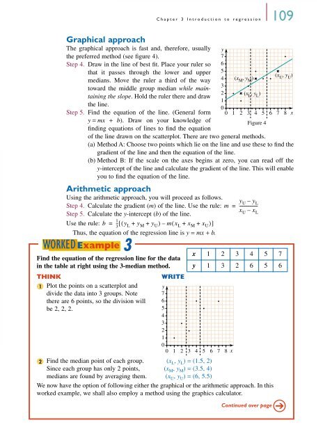
Graphical approach<br />
The graphical approach is fast and, therefore, usually<br />
the preferred method (see figure 4).<br />
Step 4. Draw in the line of best fit. Place your ruler so<br />
that it passes through the lower and upper<br />
medians. Move the ruler a third of the way<br />
<strong>to</strong>ward the middle group median while maintaining<br />
the slope. Hold the ruler there and draw<br />
the line.<br />
Step 5. Find the equation of the line. (General form<br />
y = mx + b). Draw on your knowledge of<br />
finding equations of lines <strong>to</strong> find the equation<br />
Chapter 3 <strong>Introduction</strong> <strong>to</strong> <strong>regression</strong> 109<br />
of the line drawn on the scatterplot. There are two general methods.<br />
(a) Method A: Choose two points which lie on the line and use these <strong>to</strong> find the<br />
gradient of the line and then the equation of the line.<br />
(b) Method B: If the scale on the axes begins at zero, you can read off the<br />
y-intercept of the line and calculate the gradient of the line. This will enable<br />
you <strong>to</strong> find the equation of the line.<br />
Arithmetic approach<br />
Using the arithmetic approach, you will proceed as follows.<br />
Step 4. Calculate the gradient (m) of the line. Use the rule:<br />
Step 5. Calculate the y-intercept (b) of the line.<br />
1<br />
Use the rule: b = -- [ ( y 3 L + yM + yU) – mx ( L + xM + xU) ]<br />
Thus, the equation of the <strong>regression</strong> line is y = mx + b.<br />
Find the equation of the <strong>regression</strong> line for the data<br />
in the table at right using the 3-median method.<br />
THINK WRITE<br />
1<br />
2<br />
WORKED Example<br />
3<br />
Plot the points on a scatterplot and<br />
divide the data in<strong>to</strong> 3 groups. Note<br />
there are 6 points, so the division will<br />
be 2, 2, 2.<br />
Find the median point of each group.<br />
Since each group has only 2 points,<br />
medians are found by averaging them.<br />
(x L, y L) = (1.5, 2)<br />
(x M, y M) = (3.5, 4)<br />
(x U, y U) = (6, 5.5)<br />
y<br />
7<br />
6<br />
5<br />
4<br />
3<br />
(xM , yM )<br />
(xU , yU )<br />
2<br />
1<br />
(xL , yL )<br />
0<br />
0 1 2 3 4 5 6 7 8 x<br />
m<br />
y<br />
7<br />
6<br />
5<br />
4<br />
3<br />
2<br />
1<br />
0<br />
0 1 2 3 4 5 6 7 8 x<br />
Figure 4<br />
yU – yL = ----------------xU<br />
– xL x 1 2 3 4 5 7<br />
y 1 3 2 6 5 6<br />
We now have the option of following either the graphical or the arithmetic approach. In this<br />
worked example, we shall also employ a method using the graphics calcula<strong>to</strong>r.<br />
Continued over page