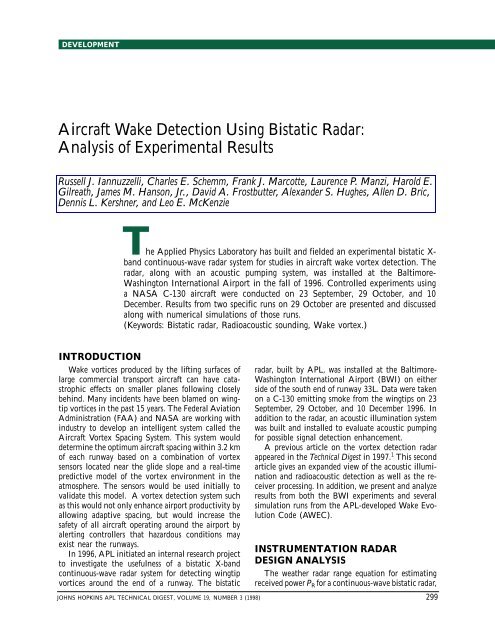
Aircraft Wake Detection Using Bistatic Radar: Analysis of ...

DEVELOPMENT 

Aircraft Wake Detection Using Bistatic Radar: 

Analysis of Experimental Results 

AIRCRAFT WAKE DETECTION 

Russell J. Iannuzzelli, Charles E. Schemm, Frank J. Marcotte, Laurence P. Manzi, Harold E. 

Gilreath, James M. Hanson, Jr., David A. Frostbutter, Alexander S. Hughes, Allen D. Bric, 

Dennis L. Kershner, and Leo E. McKenzie 

The Applied Physics Laboratory has built and fielded an experimental bistatic Xband 

continuous-wave radar system for studies in aircraft wake vortex detection. The 

radar, along with an acoustic pumping system, was installed at the Baltimore- 

Washington International Airport in the fall of 1996. Controlled experiments using 

a NASA C-130 aircraft were conducted on 23 September, 29 October, and 10 

December. Results from two specific runs on 29 October are presented and discussed 

along with numerical simulations of those runs. 

(Keywords: Bistatic radar, Radioacoustic sounding, Wake vortex.) 

INTRODUCTION 

Wake vortices produced by the lifting surfaces of 

large commercial transport aircraft can have catastrophic 

effects on smaller planes following closely 

behind. Many incidents have been blamed on wingtip 

vortices in the past 15 years. The Federal Aviation 

Administration (FAA) and NASA are working with 

industry to develop an intelligent system called the 

Aircraft Vortex Spacing System. This system would 

determine the optimum aircraft spacing within 3.2 km 

of each runway based on a combination of vortex 

sensors located near the glide slope and a real-time 

predictive model of the vortex environment in the 

atmosphere. The sensors would be used initially to 

validate this model. A vortex detection system such 

as this would not only enhance airport productivity by 

allowing adaptive spacing, but would increase the 

safety of all aircraft operating around the airport by 

alerting controllers that hazardous conditions may 

exist near the runways. 

In 1996, APL initiated an internal research project 

to investigate the usefulness of a bistatic X-band 

continuous-wave radar system for detecting wingtip 

vortices around the end of a runway. The bistatic 

radar, built by APL, was installed at the Baltimore- 

Washington International Airport (BWI) on either 

side of the south end of runway 33L. Data were taken 

on a C-130 emitting smoke from the wingtips on 23 

September, 29 October, and 10 December 1996. In 

addition to the radar, an acoustic illumination system 

was built and installed to evaluate acoustic pumping 

for possible signal detection enhancement. 

A previous article on the vortex detection radar 

appeared in the Technical Digest in 1997. 1 This second 

article gives an expanded view of the acoustic illumination 

and radioacoustic detection as well as the receiver 

processing. In addition, we present and analyze 

results from both the BWI experiments and several 

simulation runs from the APL-developed Wake Evolution 

Code (AWEC). 

INSTRUMENTATION RADAR 

DESIGN ANALYSIS 

The weather radar range equation for estimating 

received power PR for a continuous-wave bistatic radar, 

JOHNS HOPKINS APL TECHNICAL DIGEST, VOLUME 19, NUMBER 3 (1998) 299

R. J. IANNUZZELLI ET AL. 

in which the transmitter and receiver are spatially 

separated, can be shown to be 

P 

R 

2 

PGG T T R 

= v( 

VC ∩VV), 

3 2 2 

( 4) 

R R 

T R 

(1) 

where 

PT = transmitter power, 

GT and GR = transmitter and receiver antenna gains, 

respectively, 

= wavelength, 

RT and RR = ranges from the transmitter and receiver 

to the intersection of the two antenna beams, 

respectively, 

v =reflectivity of volume clutter (expressed in m2 / 

m3 ), 

VC = the common volume, which is contained within 

the intersection of the transmitter’s and 

receiver’s conical beams, and 

VV = vortex volume. 

For a monostatic radar, the ranges are identical. 

From Ref. 2, clear air turbulence reflectivity v can 

be expressed as 

4 

= 2k [ 2k sin( / 2)] 

, (2) 

v S 

where k = 2/ is the radar wavenumber, and S is the 

scattering angle, i.e., the angle at which the radar 

energy is bent at the common volume from the transmitter 

toward the receiver (180° for the monostatic 

case). The spectral representation of the turbulence is 

given by 

2 −11/ 

3 

n 

( ) = 0. 033C , 

(3) 

where is the spatial wavenumber, and 2 

C is a struc- 

n 

ture parameter that measures the intensity of turbulent 

fluctuations. For the special case of homogeneous isotropic 

turbulence, 2 

C can be expressed in terms of the 

n 

more general structure Dn(r) using 

where 

2 2/ 3 

Cn = r Dn() r 

− , (4) 

[ ] 2 

Dn() r ≡ n( x + r) − n() x 

(5) 

is the structure function, and r is a spatial increment. The 

variable n in Eq. 5 is the refractive index of air, which 

is related to meteorological variables (temperature, 

pressure, humidity). The overbar indicates an ensemble 

average. Values of 2 16 2/3 

C can range from 10 m n 

for weak turbulence to 10 12 m 2/3 for very strong 

turbulence. 3,4 

Vortex detection by radar poses several challenges 

to the radar designer. Most of the problems arise because 

the vortex provides little radar return. Since 

most of the refraction will be away from the radar 

transmitter (Ref. 1), a bistatic arrangement is favored. 

The biggest problem with the bistatic continuouswave 

radar is the performance degradation due to 

phase noise from the spillover signal. Unlike pulse 

radars, a continuous-wave radar is both transmitting 

and receiving all the time. Time gating, which isolates 

a pulse radar receiver from the transmitter, does not 

apply with a continuous-wave radar, so other means of 

isolating the high spillover signal from the transmitter 

into the receiver must be used. We applied several 

techniques to reduce spillover at BWI, including construction 

of fences around the transmitter and receiver 

shelter and separation and pointing of the receiver/ 

transmitter so that sidelobe patterns could help null 

out as much of the direct spillover as possible. In 

addition, we experimented with an active nuller 1 and 

adaptive processing, which will be described later in 

this article. Figure 1 depicts a hypothetical received 

signal spectrum, with a finite-passband noiselike vortex 

signal component, a receiver noise component, 

and a spillover component with phase noise. 

RADIOACOUSTIC DETECTION 

OF AIRCRAFT WAKES: 

ACOUSTIC PUMPING 

In 1961, the Midwest Research Institute developed 

a radioacoustic detection system, later known as RASS 

(radioacoustic sounding system), as a means for 

measuring the temperature profile of the lower 

300 JOHNS HOPKINS APL TECHNICAL DIGEST, VOLUME 19, NUMBER 3 (1998) 

Power received (dBm/Hz) 

–60 

–80 

–100 

–120 

–140 

–160 

–180 

Vortex signal 

Receiver noise 

Spillover 

Phase noise 

–200 –150 –100 –50 0 50 100 150 

Doppler frequency (Hz) 

Figure 1. Illustration of received vortex signal spectrum showing the 

major components. Turbulent fluctuations, C n 2 , were 10 12 , 10 14 , 

and 10 16 m 2/3 for strong, moderate, and weak turbulences, 

respectively. Radar specifications were transmitter power = 400 W, 

beamwidth = 1.6°, transmitter/receiver separation = 1620 m, and 

vortex height = 61 m.

atmosphere. 5 The method was later refined and extended 

elsewhere, notably at Stanford University, 6,7 in 

the former Soviet Union, 8–10 and most recently in 

Norway. 3 In such a system, acoustic waves are transmitted 

into the atmosphere to produce traveling perturbations 

in the index of refraction that can be sensed 

by a bistatic radar. The design depends on establishing 

the Bragg scattering condition, in which the RF energy 

that is scattered from successive acoustic wavefronts 

adds coherently at the receiver. For a simple collinear 

configuration, with the transmitter and receiver equidistant 

from the acoustic source (cf. Fig. 2), this condition 

occurs when 

k = 2k sin( / 2), 

(6) 

a S 

where k a is the acoustic wavenumber. 

By virtue of the movement of the scattering wavefronts, 

the frequency of the received RF signal is shifted 

by an amount equal to the Doppler frequency f d, 

which, for a quiescent atmosphere, equals the frequency 

of the acoustic source f a: 

f d = fa =− kavs , 

(7) 

where v s is the sound speed. A change in the speed of 

the wavefronts, which can be due to the advection of 

the waves by air currents or by a variation in sound 

speed, changes the Doppler frequency, and tracking 

this change is the basis for measuring wind speed or 

temperature. 

An idealized version of a radioacoustic system has 

been analyzed 2 for the case of Fraunhofer scattering 

from advecting perturbations in the refractive index. 

Applying this analysis to the configuration shown in 

Fig. 2, and arranging the results in the form of the 

bistatic radar equation, we obtain 

h 

x 

z 

Common 

volume 

s 

s /2 

Transmitter Acoustic source 

Receiver 

Figure 2. Radioacoustic detection of aircraft vortices ( s = scattering 

angle, = antenna beamwidth, and h = height.) 

( ) ( ) 

⎧ 2 2 3 4 

P= r Pg T / 

⎡ 

4 

R 

⎤⎫ 

⎨ 

⎬, 

⎩ ⎣⎢ ⎦⎥ 

⎭ 


JOHNS HOPKINS APL TECHNICAL DIGEST, VOLUME 19, NUMBER 3 (1998) 301 

(8) 

where P r = echo power, g = antenna gain, and R = 

range. 

The variable is an effective cross section (radar 

cross section of the entire volume), which is shown 

to be 

⎧ 4 

 

⎡ 2 2 

 

⎤⎫ 

C⎨ Pg a a k / 4 h ⎬, 

(9) 

⎩ ⎣⎢ ⎦⎥ 

⎭ 

= ( ) ( ) 

where P a is the power of the acoustic source, g a is the 

acoustic antenna gain, h is the distance from the acoustic 

source to the center of the common volume, the 

constant C is given by 

2 3 − 15 2 

C = 2(K )/( v ) ≈ 3. 69 × 10 m /W, (10) 

s 

and K is the Gladstone-Dale constant (see the boxed 

insert). 

For the radioacoustic configuration used in the BWI 

experiments, the acoustic line in the Doppler spectrum 

was readily detected under ambient conditions at the 

proper frequency (Fig. 3). However, the echo power 

predicted using Eq. 10 for the effective cross section 

was found to greatly exceed the level actually measured. 

The reason for the large difference is not clear, 

but it might stem from the coarseness of the initial 

theoretical approximations. The assumption of Fraunhofer 

conditions implies that the phase fronts of the 

refracted RF waves are planar throughout the common 

volume, and requires that the receiver be in the far 

field of this volume. Neither constraint is satisfied 

in the BWI configuration, but the role these factors 

play in the discrepancy remains unresolved. The limitations 

of time and scope have prevented further 

investigation. 

As noted earlier, changes in the speed of the wavefronts, 

and thereby changes in the Doppler frequency, 

can be caused either by alterations in the local speed 

of sound or by the advection of the waves by air currents 

within the common volume. Both of these effects 

occur when a vortex wake descends into the field of 

view of the radar. In general, the change in Doppler 

frequency equals 

f = − k ( v 

+w 

(11) 

d a s ), 

where the perturbation in sound speed v s depends on 

changes in temperature and composition, and w is the


THE CONNECTION BETWEEN SOUND PRESSURE LEVEL AND RADAR CROSS SECTION 

Applying the assumptions and analysis in Ref. 2, the 

variable can be related to the change in index of refraction 

induced by the sound waves by 

4 2 2 2 

=( 14 / ) k VC( nh) cos 

. 

In this equation, V C ~ (x) 3 / s is the common volume 

defined by the RF transmitter and receiver beam patterns 

in Fig. 2, and k is the RF wavenumber. The term nh is the 

amplitude of the index of refraction variations within this 

volume, which are represented as a train of plane waves, 

Acoustic 

line 

n = nhcos[ka(z vst)] , 

where v s is the sound speed and k a is the acoustic wavenumber. 

The change in index of refraction can be related to the 

acoustic pressure by 

n =K()=K(p)/v s , 

“Zero Doppler” 

spillover 

T = 63.69 s 

Figure 3. Spectrogram of run 9 on 29 October 1996 (10-kHz bandwidth). 

where K (by definition) is the Gladstone-Dale constant and 

is the air density. The acoustic pressure (p), in turn, is 

related to the intensity of the sound waves in the common 

volume by 

p =2(v s)I, 

where the intensity is given by 

I =[Paga/(4h 2 )] exp(2h). 

Here, P a is the power of the acoustic source, g a is the 

acoustic antenna gain, and h is the distance from the acoustic 

source to the center of the common volume. The variable 

is the absorption coefficient, which depends on the acoustic 

frequency, the transport properties of air, and the relative 

humidity. For the range of altitudes and frequencies of interest 

in the present work, is negligibly small, even at 

100% relative humidity. The bracketed expression given in 

Eq. 9 in the text results from using the above relationships, 

with set equal to zero. 

component of the vortex velocity 

field parallel to the acoustic axis. 

Because these variables are distributed 

nonuniformly, we might 

expect to see the Doppler spectrum 

broaden from a line to a 

continuous spectrum of width 

(f d) max as the vortex wake moves 

into the common volume. This 

was not the case, however; observations 

showed a large signal 

dropout correlating with the arrival 

of the descending wake (see the 

Results section for a discussion). 

PROCESSING 

Receiver Processing 

Figure 4 is a block diagram of 

the receiver processing. Both 

channels—the main vortex channel 

that is collecting information 

from the common volume (as well 

as spillover from sidelobes) and the 

reference channel—are mixed to 

approximately 25 kHz. From there, 

both channels are sent through a 

bandpass anti-alias filter. The data 

302 JOHNS HOPKINS APL TECHNICAL DIGEST, VOLUME 19, NUMBER 3 (1998)

Vortex 

channel 

Reference 

channel 

Center @ 25 kHz 

Anti-alias 

X bandpass 

filter 

X 

Anti-alias 

bandpass 

filter 

Center @ 25 kHz 

Oscillator Tunable 

A/D 

32K 

samples/s 

Metrum 

data 

recorder Clock 

A/D 

32K 

samples/s 

Figure 4. Receiver processing block diagram. 

Digital 

receiver 

Digital 

data 

recorder 

Digital 

receiver 

are then recorded on a Metrum RSR-512 rotary storage 

data recorder at an 80-kHz sampling rate and are 

sent for real-time data processing on a VME system at 

a sampling rate of 32 kHz. This latter rate, along with 

a downconversion/filtering scheme, will preserve up to 

8 kHz of complex digital bandwidth, depending on 

which digital filter is used. All the digital filters are 

flat for approximately 75 to 85% of the passband, with 

out-of-band rejection greater than 90 dB. The four 

different digital filters, at ±4096, 2048, 1024, 512 Hz, 

use between 128 and 512 taps. From there, a time/ 

frequency spectrogram is performed on the data, with 

a variety of time/frequency resolutions possible. The 

spectrogram, which is displayed in real time on a PC, 

is described next. 

Spectrogram Processing and Display 

Briefly, a spectrogram is a specific type of time/ 

frequency distribution based on the periodogram, with 

extensions built in for time resolution. Many types of 

time/frequency distributions have received much attention; 

however, for real-time display, none can compare 

to the fast Fourier transform (FFT)-based distribution 

in terms of computational speed. 

Figure 5 is a block diagram of overlapping FFT 

processing known as the spectrogram. After the digital 

receivers, the complex data are buffered. This allows 

the FFT to be overlapped by any 

desired amount. Three parameters 

control the spectral processing. (1) 

FFTsize is the size of the FFTs used 

(typically 256, 512, or 1024 

points). (2) FFTdsize is the data 

size portion of the FFTsize. Typically, 

this is at most the FFTsize or 1 

to 2 powers of 2 smaller. This parameter, 

along with the sampling 

rate and the specific digital filter 

used in the digital receiver, will 

establish the spectral resolution. If 

I/Q 

data 

Data buffering 

several seconds 

of data 

Spectral 

and 

adaptive 

processing 


a windowing function is used, it 

may also affect the resolution. (3) 

FFTndsize is the new data size 

portion of the FFTdsize for FFT 

processing, which will typically be 

at most the FFTdsize or perhaps 1 

to 4 powers of 2 smaller. This parameter 

will establish the time resolution 

of the spectrogram. In addition 

to these parameters, the 

noise floor parameter can be set to 

between 10 and 150 dB, and 

variable infinite impulse responsetype 

averaging can be performed 

on the postmagnitude operation. 

Figure 3 is an example of the 

spectrogram for run 9 on 29 October, with FFTsize = 

1024, FFTdsize = 512, and FFTndsize = 128 in a digital 

bandwidth of ±5000 Hz. With these parameters set, 

along with a Hanning windowing scheme that reduces 

the spectral resolution, the spectral resolution is approximately 

15 Hz. The time resolution is approximately 

0.13 s, since this is the amount of spectral 

integration that occurs between successive FFTs. In 

Fig. 3, time progresses downward, where extent of the 

time scale is a function of the number of graphics pixels 

in the display window. With a 1024 768 display 

mode set, this window yields approximately 78 s of 

simultaneously viewable spectrogram data. The interpretation 

of the data will be discussed in the Results 

section. 

Adaptive Processing 

The spillover from the transmitter to the receiver 

is several orders of magnitude larger than any atmospherically 

based signal reflected down from the common 

volume. This makes any detections close to the 

zero-Doppler frequency difficult to obtain. To cancel 

some of the spillover, the reference channel is used to 

adaptively cancel anything that is common. Illuminator 

phase noise is common to both channels and thus 

should cancel, whereas the vortex signal, which is not 

contained in the reference channel, should become 

FFTdsize 

data 

points 


FFT 

Display 

FFTsize 

data 

points 

FFTndsize Possible 

zero padding 

Windowing 

Complex data 

Output FFT line 

(FFTndsize* sample 

period in seconds) 

Real data 

IIR 

filter 

Average 

time constant 

20 log ( ) 

Lower 

limit 

Figure 5. Block diagram of spectrogram FFT processing (IIR = infinite impulse 

response).


more apparent after adaptive processing. 

The formulation for this 

adaptive process assumes that the 

main vortex channel has two components: 

the common volume 

component and the direct spillover 

component. The reference 

channel is first phase-shifted and 

scaled to match the zero-Doppler 

magnitude and phase of the vortex 

channel peak, and then subtracted. 

The subtraction is performed in 

the frequency domain before the 

magnitude is taken. This has typically 

reduced the power in the 

zero-Doppler component in the 

main vortex channel by as much as 

30 dB. Figure 6 is a block diagram 

of the adaptive processing, which 

Vortex 

I/Q 

data 




can be contrasted to the spectrogram processing depicted 

in Fig. 5. Many runs were looked at with this 

process, and for those of importance on 29 October, 

adaptive processing was not needed since the returns 

were quite large. 

THE BWI EXPERIMENT 

Both the Maryland Aviation Administration and 

the FAA where extremely helpful and receptive to the 

idea of allowing APL to install and operate the bistatic 

radar on the south side of runway 33L (Fig. 7). As 

mentioned previously, because of the proximity of the 

test site to a highway, wire screen fences (Fig. 8) were 

installed around both locations. This cut down reflections 

from cars as well as the direct path signal from 

the transmitter to the receiver. 

The traffic interference can be recognized in waterfall 

spectra as a double S-shaped curve with an inflection 

point at zero Doppler (Fig. 3). This region of zero 

Doppler occurs when the vehicle is midway between 

the transmitter and receiver and the rate of change of 

the sum of the ray paths from the transmitter and the 

receiver to the vehicle is zero. At times prior to this 

there is a decreasing positive rate of change (positive 

Doppler); after the midway point there is an increasing 

negative Doppler. The maximum positive and negative 

velocity is limited to that of a monostatic radar 

with a completely radial component. Traffic interference 

can be seen in the actual waterfall data of Fig. 

3 as depicted in Fig. 9. 

Initial checkout of the system consisted of antenna 

alignment testing followed by measurement of receiver 

signal levels in clear air, both with and without acoustic 

pumping. Also, with the runway out of service, the 

acoustic transmitter was moved to several locations 

along its centerline, and receiver signal levels were 

Windowing 

20 log ( ) 


FFT 

FFTndsize Possible 

zero padding 




Reference 

I/Q 

data 

FFTdsize 

data 

points 

FFT 

FFTsize 

data 

points 

Complex data 

Reference channel 

phase-shifted and 

subtracted from main 

vortex channel 

Real data 

IIR 

filter 

Average 

time constant 

Figure 6. Block diagram of adaptive spectrogram FFT processing. 

Output FFT line 

(FFTndsize* sample 

period in seconds) 

Lower 

limit 

monitored. During this phase of testing, the acoustic 

transmitter consisted of a Peavy 44T compression driver 

loaded with a 60° horn, which was typically driven 

with less than 20 W. A digital synthesizer was used to 

generate a sinusoidal input to the amplifier, which 

could be varied in frequency. 

Tests confirmed that the optimal orientation of the 

acoustic source was vertical and directly in line between 

the transmitter and receiver along the centerline 

of the runway; i.e., at about 79 m from the south 

end of the runway. Unfortunately, commercial aircraft 

are at a very low altitude as they pass over this point, 

perhaps ≈50 m or less. At this altitude, a vortex can 

be unstable and dissipate quickly. To allow better control 

of the test environment, arrangements were made 

for a NASA C-130 aircraft from Wallops Island, Virginia, 

to overfly the runway on several days. These 

flights were funded by NASA as a contribution to the 

APL research efforts. 

Test Aircraft 

The C-130 aircraft was equipped with smoke 

generators (smokers) installed on both wingtips. The 

smokers burned corvus or canopus oil at the wingtip, 

which caused the smoke to became entrapped in the 

vortex core (see Fig. 10). The entrapped smoke allowed 

visual tracking of the otherwise invisible vortex. 

The right-tip smoker was inoperative for the first two 

test dates owing to a defective switch in the cockpit; 

however, both tip smokers were operational during the 

third and final test date. 

Pretest instructions required the C-130 crew to fly 

the glide slope until reaching the requested altitude, 

which was to be held until the aircraft passed 305 m 

beyond the runway threshold. To conserve the corvus 

oil, the smoke was to be turned on 305 m prior to the

(a) 

Runway 33L 

MD Rte. 176 Receiver Transmitter 

(b) 

Receiver 

Radar fence 

Touchdown area 

Runway 

33L 

Acoustic 

pumping 

device 

runway threshold and turned off 305 m beyond the 

threshold. A NASA video of the C-130 taken during 

a previous test at Wallops Island revealed that the tip 

vortices would break up if the landing flaps were used. 

Therefore, the C-130 was instructed to fly by the APL 

test sight in a “clean” configuration (gear and flaps up) 

at a speed of 1.3 Vso (120–130 kt). (Vso = stall speed 

or minimum steady flight speed at which the aircraft 

is controllable in the landing configuration.) At this 

speed and at maximum fuel weight, the strength of the 

vortices generated by the C-130 equaled that generated 

by a Boeing 727. 

Radar fence 

Transmitter 

15–120-m 

common 

volume 

height 

600-m 

transmitter/receiver 

separation 

Figure 7. BWI vortex detection test site on runway 33L: (a) aerial photograph and (b) 

schematic view. 

Figure 8. Wake vortex receiver at BWI. 


During the test, the C-130 received 

instruction via a UHF radio 

that was based at the radar receiver 

location. APL would transmit altitude 

and lateral displacement instructions 

to the crew before each 

flyby. The co-pilot received instructions 

from the APL test site, 

while the pilot communicated 

with the control tower at BWI. 

Data Collection Procedures 

A typical run of the C-130 involved 

at least six people: four at 

the receiver container, one at the 

transmit container, and one at the 

acoustic site. One person (local 

controller) was in voice communication 

with the C-130 at all times. 

The local controller and at least 

three other people were at the receiver 

container and would specify 

a height above the runway and 

distance from side to side offset 

from the runway to the crew. A 

“mark” would be given to the two 

or three people manning the receiver 

equipment that the C-130 

was about 305 m out. Data collection 

usually started at this point. 

Visual contact was also made by 

the person voice-annotating the 

Metrum data. The receiver container, 

the transmit container, 

and the person manning the 

acoustic illuminator were all in 

radio communication. The person 

at the acoustic setup, which was 

in-line with the runway, would 

give a mark when the C-130 was 

over Dorsey Road and then when 



20 

0 

Time (s) 40 

–20 

–40 

–1500 –1000 –500 0 500 1000 1500 


Figure 9. Interference shown for a vehicle traveling 40 mph on 

Rte. 176. 

over the common volume. At this point, most of the 

voice annotation centered on the vortex smoke trails 

as seen by the receiver video camera. When the transmit 

container saw smoke in the transmit monitor, radio 

contact was made and notes taken at the receiver 

container specifying the degree of visual collaboration 

of smoke in the cameras at the receiver and transmit 

sites. This procedure worked well in establishing which 

of the many data runs were worth further investigation. 

Observed Vortex Behavior 

The behavior of the wingtip vortices was videotaped 

during the three test periods. Near-surface temperature 

and wind data were recorded at the radar 

receiver site. Recording devices were not allowed near 

or above the runway surface. Operations during the 

evening hours provided the most stable atmospheric 

conditions for the first test period. Because of the time 

change to Eastern Standard Time after the first tests 

and the heavy airline activity, the second and third 

tests were conducted during the morning and afternoon 

hours. A general description of the wind conditions 

and the vortex behavior during each test period 

is given in the following paragraphs. 

The first test began at 5:20 p.m. on 23 September. 

Winds were 5 to 10 kt along the runway centerline. 

The C-130 made 20 passes by the APL test site at 

altitudes ranging from 15 to about 107 m above ground 

level (AGL). As noted earlier, the left wingtip smoker 

worked, but the right tip had malfunctioned. The lefttip 

vortex lasted more than 2 min after the C-130 flyby. 

The vortex remained near the runway centerline at 

approximately 12 m AGL. In some cases, the vortex 

passed through the boresight camera’s view and would 

reappear shortly thereafter, giving the false impression 

that the vortex was rising. Instead, it remained near 

about 12 m AGL but underwent a wavelike oscillation. 

The peak of the wave motion reappeared in the boresight 

camera’s view. 

The first test date provided the best atmospheric 

conditions for vortex longevity, but posttest analysis 

determined that the radar’s common volume was too 

low and the local traffic on Dorsey Road caused too 

much interference in the radar data. 

The second test started at 9:50 a.m. on 29 October. 

Again, the right-tip smoker had malfunctioned. Initially, 

winds were approximately 15 to 20 kt across the 

runway. In some cases, the C-130 was instructed to fly 

at two wingspans about 80 m to the right of the runway 

centerline in hopes that the vortices would pass 

through the radar’s common volume. After six passes, 

the winds decreased to light and variable and the 

C-130 was instructed to fly over the runway centerline. 

Fifteen passes were made by the C-130 until the BWI 

tower terminated testing owing to increasing commercial 

air traffic. The second half of this test provided the 

best radar data. 

The third and final test date was 10 December. The 

malfunction in the right-tip smoker had been corrected, 

thereby allowing the observation of the interaction 


(a) 

(b) 

Figure 10. The NASA C-130 research aircraft with generator on 

left wing. (a) Trailing vortex seen on approach to BWI. (b) Smokemarked 

vortex as seen several seconds after the C-130 passed 

by (a).

etween the left and right vortices. The C-130 was 

committed to a full day of testing, which included a 

landing at BWI with the smokers on. Wind conditions 

were less than ideal, with estimated crosswinds at 

velocities of 20 to 25 kt. Lateral positioning of the C- 

130 was difficult owing to the variation in the wind 

velocity and direction. Even under these conditions 

the tip vortices would remain intact for over 1 min. 

The vortices appeared in the boresight camera’s view 

for only a few seconds because of the lateral displacement 

caused by the crosswinds. 

Testing on 10 December began at 10:19 a.m. The 

C-130 made 13 passes before the BWI controllers terminated 

the test because of an increase in commercial 

air traffic. At this time, the C-130 landed for refueling 

with the smokers on. The tip vortices were destroyed 

within two C-130 body lengths, with the landing flaps 

fully deflected. 

Afternoon testing began at 1:35 p.m. The winds 

had not subsided, and lateral positioning remained a 

problem. The radar’s common volume was moved in 

an attempt to track the vortices as they were displaced 

by the crosswinds. At 3:00 p.m., the C-130 made its 

40th and final pass of the afternoon and returned to 

Wallops Island. 

RESULTS 

No significant Doppler signatures could be correlated 

with the times and runs when smoke was seen in 

the video cameras on 23 September or 10 December. 

On the earlier date, the common volume was at 15 m, 

which we later realized was a poor choice because of 

ground effects. On 10 December, the winds made it 

difficult to impossible to position the C-130 so that 

smoke would drop through the common volume. 

Two data runs taken on 29 October are detailed in 

the following paragraphs. Both proved to have definitive 

Doppler signatures when smoke was observed to 

be dropping through the common volume. (A more 

detailed presentation of the data from all the runs may 

be found in Ref. 11.) 

The radioacoustic return showed a large signal 

dropout correlated with the arrival time of the descending 

wake (cf. Fig. 11a). The major qualitative 

difference between these results and the simplified 

picture presented earlier is likely due to a combination 

of effects associated with three phenomena: 

1. Wake turbulence. Fluctuations in velocity and temperature 

distort the acoustic wavefronts, scattering 

the acoustic power and causing a loss of coherence in 

the wavetrain. 

2. Cross-currents. Velocity components perpendicular 

to the acoustic axis tilt the Bragg grid, changing its 

geometry with respect to the RF beams, and possibly 

de-tuning the system. 


3. Vertical shear. The presence of shear means that 

waves are advected by differing amounts in different 

parts of the wavetrain. When the acoustic axis is 

vertical, the fractional change in wavenumber along 

a central ray is directly proportional to ∂ w/∂ s, i.e., 

∂( ln k)/ ∂s = −∂w/ ∂s/( 

v + w), 


s 

(12) 

where s is the distance along the ray. The resulting 

refraction is strongest in the core region of the vortices 

and would tend to de-tune the system when the cores 

occupy the common volume. 

Recall Fig. 3, a spectrogram of the data from the 

main vortex channel from run 9 (time running from 

oldest to newest, top to bottom). Figure 11b is a reduced 

bandwidth view of the same run. Here the frequency 

resolution is approximately 1 Hz as opposed to 

15 Hz in Fig. 3. Marks have been added to the time axis 

where the smoke was observed in the cameras. 

A Doppler event within these marks is evident and is 

believed to represent the drop rate of the vortex core. 

The positive side of the Doppler spectrum corresponds 

to the “drop side” Doppler, i.e., the path length is being 

shortened. Calculations of the drop rate from the receiver 

video after the fact seem to generally agree with 

the drop rate indicated by the spectrogram and with the 

results of the numerical model calculations (cf. Fig. 15). 

Knowing the video camera’s field of view and the 

approximate distance to the smoke, the video drop rate 

was estimated to range from 1.3 to 3.5 m/s. This corresponds 

to a Doppler frequency at the specific X-band 

frequency used of approximately 30 Hz (2 m/s). 

Figure 11c is a cut through the spectrogram at the 

time when the vortex signature was the strongest. 

From this figure, the estimated Doppler offset is approximately 

40 Hz. Two other traces are depicted here, 

2 

attempting to place bounds on Cn using different 

measurement methods. The top trace (upper bound) 

assumes that the full common volume (about 1000 m3 ) 

2 

is contributing to Cn , and the energy is concentrated 

in the narrow frequency band of the vortex signal 

shown in the figure. The bottom trace (lower bound) 

assumes that the received energy is spread over the 

frequency band corresponding to the estimated turbulent 

velocities contained in the vortex. The figure 

2 

shows that Cn is several orders of magnitude greater 

than the upper bound, suggesting that vortices may 

2 

have Cn values much greater than expected for 

strong, clear air turbulence. Another explanation is 

that the smoke contained in the vortex is contributing 

to overall vortex reflectivity. Compare Fig. 11c with 

Fig. 11a, a peak amplitude versus time plot for the 

acoustic line. Here, the dropout from the passage of the 

plane is apparent; however, little else could be counted 

on because of the wide swings in received power.


(a) 

Acoustic tone spectral power (dB) 

–30 

–40 

–50 

–60 

–70 

–80 

–5 0 5 10 15 20 25 30 35 40 45 

Elapsed time from C-130 overflight of common volume (s) 

(b) 


spillover 

Vortex 

signature 

Figure 12 shows the acoustic amplitude, spectrogram, 

and single line spectrum for run 15. Again, the 

reader will find details on additional runs in Ref. 11. 

MODEL PREDICTIONS OF AIRCRAFT 

VORTEX WAKES 

Model calculations have been carried out for runs 

9 and 15 from 29 October. Our objectives were (1) to 

determine the extent to which the model could predict 

the early evolution (prior to breakup) of aircraft vortices 

and (2) to help interpret the radar measurements 

described in previous sections. 

Iannuzzelli-11a 

T = 63.69 s 

Obviously, some success in model validation is required 

if the model is to be used to provide estimates 

of the location, strength, and internal structure of the 

atmospheric flow signatures believed to be responsible 

for the measured radar returns. Accordingly, our approach 

was to first examine the predicted wake vortex 

trajectories and then to compare the predicted time of 

arrival of the vortex cores at the radar common volume 

with the time at which radar signatures were observed. 

Since no ground-truth measurements of atmospheric 

motions were available during the BWI experiment, 

these were the only comparisons that could be used to 

help establish the model’s credibility. The next step in 


Spectral power (dB) 

–20 

–60 

–80 

–100 

–100 

–50 

Spillover 

C 

–40 

2 = 10 –12 n full 

volume; power across 

measured band 

Vortex signal 

2.2 m/s 

Phase noise 

0 50 


C 2 = 10 –12 n vortex volume; 

power across 

vortex circulation 

Figure 11. Run 9 on 29 October 1996: (a) acoustic line power, (b) spectrogram, and (c) single line through spectrogram. 

(c) 

100 

150

Acoustic tone spectral power (dB) 

(a) 

–30 

–40 

–50 

–60 

–70 

–80 

0 10 20 30 40 

Elapsed time from C-130 overflight of common volume (s) 

(c) 


spillover 

the analysis process was to examine features of the 

predicted vortex wakes (e.g., overall size, internal 

structure) to better understand what parts of the signature 

might be responsible for the measured radar 

returns. 

Predictions of vortex wake evaluation were obtained 

using the recently developed APL Wake Evaluation 

Code (AWEC). AWEC solves steady-state r non- 

linear equations for the velocity 

V, density , 

turbulence kinetic energy K, and turbulence dissipation 

rate , all in a coordinate system that is fixed with 

respect to a moving source (in this case, an aircraft) 

Vortex 

signature 

T = 31.85 s 


and moves linearly with that source. A second-order 

turbulence closure scheme, based largely on the Mellor 

and Yamada Level 2.5 model, 12 is used to evaluate the 

remaining turbulence correlations. 

The principal approximation in AWEC, and the 

one that renders the problem tractable, is the so-called 

parabolic approximation. The physical assumption 

behind this approximation, which is valid for almost 

all wake flows, is that changes in the downtrack or x 

direction are small compared with changes in the 

crosstrack and vertical (y and z) directions. Derivatives 

of x other than those in advective terms involving the 


Spectral power (dB) 

–20 

–40 

–60 

–80 

–100 

–100 

–50 

Spillover 

C 2 = 10 –12 n full 

volume; power 

across 

measured band 

0 

Vortex signal 

~4.8 m/s 

Phase noise 

50 

100 


Figure 12. Run 15 on 29 October: (a) acoustic line power, (b) spectrogram, and (c) single line through spectrograph. 

(b) 

C 2 = 10 –12 n vortex 

volume; power 

across vortex 

circulation 

150 

200


mean speed of advance U are neglected, thereby allowing 

the equations to be reformulated and solved as a 

marching problem in x. The need to store model 

variables at locations along the x axis is eliminated, 

thus reducing the problem from three to effectively 

two spatial dimensions. 

To initialize AWEC model calculations, estimates of 

data are needed at a vertical (y–z) plane close to the 

origin. For submarine wake predictions, a separate 

program, FWI, 13 is used to generate estimates of component 

wakes for the many sources that contribute to 

the composite wake signature. FWI stores relevant 

geometrical variables for different submarines and uses 

these values along with operating conditions provided 

by the user to compute estimates for variables such as 

the size and strength (circulation) of vortices shed by 

the hull and control surface. For the present aircraft 

vortex calculations, it was a fairly straightforward 

exercise to add a file containing the wingspan and 

other relevant geometrical variables for a C-130 transport 

and to use existing software to calculate the required 

initial plane data. Since the inviscid theory 

applied to derive the vortex circulation equations in 

FWI was originally developed for the aircraft vortex 

problem, there was little risk in applying those same 

equations to the problem at hand. And since, unlike 

submarine wakes, aircraft wakes are dominated by a 

single component, all sources other than wing vortices 

could safely be ignored. 

Run 9 

During run 9, the aircraft was assumed to be in level 

flight at an altitude of 83.8 m, with an air speed U of 

64.3 m/s. The plane’s weight was taken to be 143,000 

lb (64,865 kg), and the lift force L was assumed equal 

and opposite to the weight. The wingspan B was about 

40.4 m. 

The initial vortex circulation 0 was estimated 

from the inviscid theory. Assuming elliptical loading, 

0 

= L 

Ub 

0 

2 

= 312 ms / , (13) 

where the density of air = 1 kg/m 3 , and the vortex 

core separation b 0 is given by 

 

b 0= 

B= 31. 7 m. (14) 

4 

The diameter of the vortex core D V is given theoretically 

by 

D V = 0. 197b0 , 

(15) 

which yields an estimate of D V = 6.25 m for the 

C-130. This value was considerably larger than the 

observed core diameter of approximately 1 m. The 

latter value was determined by the visible boundary of 

the entrained smoke in the photographs. Despite this 

discrepancy, the larger theoretical value was used in 

the model calculations. Use of the smaller value would 

have required a minimum grid separation distance 

much smaller than the 0.5 m used in the present 

calculations, which would have resulted in a nearly 

prohibitive increase in the computational burden. 

The net downward vertical velocity w 0 induced by 

one vortex acting on another is given by 

−Γ 

w 0= 

2b 


0 

0 

=−157 

. m/s . (16) 

The atmosphere was assumed to be weakly stratified 

with a potential temperature gradient of 6.7 10 3 

°C/m. Values of potential temperature were converted 

to density for use by AWEC. Ambient levels of turbulence 

kinetic energy and turbulence kinetic energy 

dissipation rate were chosen to be 0.1 m 2 /s 2 and 2 

10 3 W/kg, respectively. 

Figure 13 depicts vector velocities at times late t of 

1.4 (the initial plane), 9.0, 21.0, and 31.0 s. Since the 

wing was positioned near the top of the fuselage (effective 

diameter of approximately 5.2 m) on the 

C-130, the vortex cores initially were situated 86.4 m 

AGL. Figure 14 shows contours of the turbulence 

kinetic energy for two of these times late, 1.4 and 31.0. 

The position of the radar common volume, which is 

centered at 45.7 m AGL, is also shown. 

Figure 15a plots the position of the vortex cores 

(solid curve) as a function of t. The heavy dashed line 

indicates where the vortex positions would be if the 

wake descended at a constant velocity given by the 

induced velocity computed from Eq. 16. The actual 

vortex descent begins near this speed but then slows. 

The fixed upper and lower boundaries of the common 

volume are indicated by a pair of solid horizontal lines. 

The outlying lighter dotted lines indicate the first 

contour level above ambient of the turbulence kinetic 

energy distribution. 

From Fig. 15a it is estimated that the leading edge 

of the vortex wake first reached the common volume 

approximately 12 s after aircraft passage and that the 

vortex cores were within the common volume between 

t ≈ 29 and 33 s after aircraft passage. Radar results discussed 

previously show a distinct signature at t = 31 s, 

which appears consistent with the model prediction. 

This result, however, could be fortuitous as it depends 

on the aircraft altitude at the time of passage, and there 

is considerable uncertainty in the estimates of altitude 

obtained from the C-130 pilot.

(a) (b) 

120 

120 

Height (m) 

100 

80 

60 

40 

20 

Run 15 

0 

–60 –40 –20 0 20 40 

Crosstrack (m) 

(c) (d) 

Height (m) 

120 

100 

80 

60 

40 

20 

0 

–60 –40 –20 0 


20 40 

Figure 13. Run 9 vector velocities at times late of (a) 1.4 s, (b) 9.0 s, (c) 21.0 s, and (d) 31.0 s. 

Except for the altitude, all model inputs for run 15 

were the same as those for run 9. Although the reported 

altitude was 64 m, a video tape of the aircraft 

flying over the common volume shows that the vortex 

cores as measured by smoke are in the common volume 

at the time of passage. Accordingly, an initial vortexcore 

height of 53.3 m was adopted for the run 15 model 

calculation, which resulted in better agreement with 

experimental data. 

Figure 15b plots the position of the vortex cores as 

a function of time. Again, the actual vortex motion 

descent rate is slower than predicted by inviscid theory. 

Vortex cores are predicted to be within the common 


0 

–60 –40 –20 0 


20 40 

volume between 6 and 12 s after aircraft passage. This 

agrees with the radar observations—an expected result 

here since the radar data along with the video were 

used to estimate the initial altitude. 

DISCUSSION 

Radio waves are scattered by turbulent irregularities 

in the refractive index of air. In the initial stages of a 

turbulent mixing process, air parcels are rapidly displaced 

from each other and their identities are preserved. 

It takes a while for diffusion to act and for the 

mixed region to become nearly homogeneous again. 

The stronger the initial gradients and the turbulence, 


Height (m) 

Height (m) 

100 

80 

60 

40 

20 

120 

100 

80 

60 

40 

20 

0 

–60 –40 –20 0 


20 40


(a) 

Height (m) 

(b) 

Height (m) 

120 

100 

80 

60 

40 

20 

0 

–60 –40 –20 0 


20 40 

120 

100 

80 

60 

40 

20 

0 

–60 –40 –20 0 


20 40 

Figure 14. Contours of turbulence kinetic energy for run 9 at 

times late of (a) 1.4 s, and (b) 31.0 s. 

the larger are these temporary local variations in the 

refractive index. 

The physical variable most identified with radar 

signatures is the structure parameter 2 

C discussed pre- 

n 

viously. To effectively use the model predictions to 

interpret the radar observations, a means must be 

found to relate 2 

C to the mean-flow and turbulence 

n 

variables predicted by AWEC. 

An algebraic expression for 2 

C in terms of selected 

n 

AWEC model variables has been derived for a special 

case of zero moisture content in the atmosphere, 11 

2 2 

2 a ( 77. 6R) 

Cn= − ′ v′ 

w , 

1/3 4 

10 

y z 

∂ ⎛ ⎞ 

⎜ − ′ 

′∂ ⎟ 

⎝ ∂ ∂ ⎠ 

60 

60 

(17) 

Figure 15. Vortex trajectories for (a) run 9 and (b) run 15. The 

position of the vortex cores (solid curve) is plotted as a function of 

time late. The heavy dashed line indicates where the vortex 

positions would be if the wake descended at a constant velocity 

given by the induced velocity computed from Eq. 16. The actual 

vortex descent begins near this speed but then slows. The fixed 

upper and lower boundaries of the common volume are indicated 

by a pair of solid horizontal lines. The outlying lighter dotted lines 

indicate the first contour level above ambient of the turbulence 

kinetic energy distribution. 

where is the turbulence dissipation rate, ′ v ′ and 

′ w ′ are turbulence density-velocity correlations, and 

∂/ ∂y 

and ∂/ ∂z 

are gradients of the mean potential 

density14 in the horizontal (cross-track or y) and vertical 

directions, respectively. Constants appearing in 

Eq. 17 are the universal gas constant R and a2 , which 

ranges between 0.4 and 4. A value of a2 = 1.0 was 

2 

chosen for estimating Cn in this study. 

Figure 16a shows that the wake boundary as determined 

by the structure parameter roughly coincides 

with the outer contour of turbulence kinetic energy for 

run 15, which is shown for comparison in Fig. 16b. 

Unlike the turbulence kinetic energy, however, the 

2 

plot of Cn shows evidence of structure within the 

vortex wake. Values of 2 

C range from 30 to 70 dB 

n 

over the extent of the recirculation cell, with the 


Height (m) 

(a) 

(b) 

Height (m) 

120 

100 

80 

60 

40 

20 

0 

0 

120 

100 

80 

60 

40 

20 

0 

0 

20 

20 

Time (s) 

Time (s) 

40 

40 

60 

60

(a) 

Height (m) 

120 

100 

80 

60 

40 

20 

2 

Cn (dB) 

–30 

largest values occurring near the vortex cores. The plot 

of 2 

C also shows a well-defined leading edge of the 

n 

wake. 

It is unclear whether mean velocities (as measured 

by the vector plots) or turbulent perturbations to the 

refractive index (as measured by the structure parameter) 

are primarily responsible for the observed radar 

signatures. The coincidence of regions of high velocity 

with regions of high 2 

C in the model predictions 

n 

makes it difficult to use model predictions to resolve 

this issue. 

The interpretation of the radar measurements is 

also made difficult by the absence of ambient 

crosstrack wind data. The model predictions, which 

assumed no ambient wind, show most of the vortex 

wake (including both cores) passing through the radar 

common volume; however, even a modest crosstrack 

wind could cause an offset that could result in only one 

of the cores being detected. In the former case, the 

large rotational velocities would likely be averaged 

–40 

–50 

–60 

0 

–60 –40 –20 0 20 40 

–70 

60 

(b) 


Height (m) 

120 

100 

80 

60 

40 

20 

0 

–60 –40 –20 0 20 40 


Figure 16. Run 15 at 9.0-s time late: (a) gray-scale plot of C n 2 and 

(b) contours of turbulence kinetic energy. 

60 


out, leaving only the much smaller (≈1 m/s) net downward-migration 

velocity to be measured. In the latter 

case, the radar could be detecting the composite of the 

vortical velocity and the migration velocity, which, 

according to the model predictions, could be as high 

as 7.4 m/s in regions where the two components add. 

Clearly, future experiments would benefit by direct 

measurements of the atmospheric variables of interest. 

SUMMARY 

APL has designed and constructed a bistatic continuous-wave 

radar system for experimentation in aircraft 

wake vortex detection. Many hurdles, both technical 

and logistical, were overcome in developing the 

facility. Acoustic pumping was evaluated as a possible 

technique to enhance overall detection performance. 

The radar and acoustic systems were installed at BWI 

in the fall of 1996, and controlled experiments using 

a NASA C-130 aircraft were conducted. 

From these experiments, Doppler signatures from 

the main vortex signal were found in several data runs. 

The acoustic signal showed amplitude dropouts that 

coincided with the passage of the aircraft through the 

common volume and could be used for a coarse, but 

unreliable, detection of vortex passage. We speculate 

that with the wider-band acoustic illumination, Doppler 

phase modulations will also be visible. 

APL has carried out a number of wake vortex simulations 

in support of these experiments. Model results 

have been used to help interpret the data observations. 

Predicted vortex trajectories were found to agree with 

the data when uncertainties in the aircraft altitude 

were taken into account. The model predictions have 

also provided insight into which part of the overall 

wake signature might be producing the observed radar 

returns. 

The main result from these experiments is that 

vortices are detectable with the APL X-band bistatic 

radar system. In addition, given the tremendous volume 

that must be scanned in an operational environment, 

the current system parameters (power, resolution) 

appear to be more than suitable for a fieldable 

vortex detection radar. 

One possible future direction would be to add the 

ability to track vortices in and around the end of the 

runway. This, along with a search mode, would be 

required to make the current radar a valuable sensor 

in an operational environment. Another possibility 

would be to add a millimeter-wave radar, since modeling 

has shown that it may be possible to observe 

intercore velocities with shorter wavelengths. Finally, 

we would like to extend our experimentation with 

various acoustic waveforms and techniques to further 

our understanding of the radioacoustic effects. 



REFERENCES 

1 Hanson, J. M., and Marcotte, F. J., “Aircraft Wake Vortex Detection Using 

Continuous-Wave Radar,” Johns Hopkins APL Tech. Dig. 18(3), 348–357 

(1997). 

2 Doviak, R., and Zrnic, D., Doppler Radar and Weather Observations, 2nd Ed., 

Academic Press, San Diego, CA (1993). 

3 Measurement of Atmospheric Parameters with a Bistatic Radar Supplemented by 

an Acoustic Source, Environmental Surveillance Technology Programme, 

Oslo, Norway (Oct 1995). 

4 Stewart, E. C., A Study of the Interaction Between a Wake Vortex and an 

Encountering Airplane, AIAA Paper 93-3642, Atmospheric Flight Mechanics 

Conference, Monterey, CA (Aug 1993). 

5 Smith, P. L., Jr., Remote Measurement of Wind Velocity by the Electromagnetic 

Acoustic Probe, Midwest Research Institute, Kansas City, MO (1961). 

6 Marshall, J. M., Peterson, A. M., and Barnes, A. A., Jr., “Combined Radar- 

Acoustic Sounding System,” Appl. Opt. 11(1), 108–112 (Jan 1972). 

7 Frankel, M. S., and Peterson, A. M., “Remote Temperature Profiling in the 

Lower Troposphere,” Radio Sci. 11(3), 157–166 (Mar 1976). 

8 Kon, A. I., “A Bi-Static Radar-Acoustic Atmospheric Sounding System,” 

Izvestiya (Atmospheric and Ocean Physics) 17(6), 481–484 (1981). 

9 Kon, A. I., “Signal Power in Radioacoustic Sounding of a Turbulent 

Atmosphere,” Izvestiya (Atmospheric and Ocean Physics) 20(2), 131–135 

(1984). 

CONTRIBUTORS 

10 Kon, A. I., “Combined Effect of Turbulence and Wind on the Signal 

Intensity in Radioacoustic Sounding of the Atmosphere,” Izvestiya (Atmospheric 

and Ocean Physics) 21(12), 942–947 (1985). 

11 Iannuzzelli, R. J., Marcotte, F. J., Hanson, Jr., J. M., Manzi, L. P., Schemm, 

C. E., et al., Final Report: Results of the APL Bistatic X-Band Vortex Detection 

Radar from C-130 Flyovers at BWI Airport, JHU/APL, Laurel, MD (1997). 

12 Mellor, G. P., and Yamada, T., “Development of a Turbulence Closure 

Model for Geophysical Fluid Problems,” Rev. Geophys. Space Phys. 20, 851– 

875 (1982). 

13 Rosenberg, A. P., FASTWAKE Initialization and Flow Evolution Program 

User’s Guide, STD-R-1577, JHU/APL, Laurel, MD (Nov 1987). 

14 Gill, A. E., Atmosphere-Ocean Dynamics, Academic Press, New York (1982). 

ACKNOWLEDGMENTS: The authors gratefully acknowledge the 

contributions of Robert Neece and Ann McKenzie, NASA, Langley, 

C-130 funding; Doug Young and the C-130 crew at NASA, Wallops 

Island; Ben Martinez, MAA, BWI; and Jerry Dudley, FAA, BWI. 

The BWI experiment would not have been possible without the 

diligent efforts of Bernie Kluga and Bob Geller and the air traffic 

controllers of the FAA at the BWI Tower. 

(Back row, left to right) David A. Frostbutter, William R. Geller, Laurence P. Manzi. 

(Front row, left to right) Charles E. Schemm, Harold E. Gilreath, Russell J. Iannuzzelli, James 

M. Hanson, Jr., Frank J. Marcotte, Dennis L. Kershner, Alexander S. Hughes, Allen J. Bric, 

Bernard E. Kluga. Leo E. McKenzie is not pictured. 

314 JOHNS HOPKINS APL TECHNICAL DIGEST, VOLUME 19, NUMBER 3 (1998)

Aircraft Wake Detection Using Bistatic Radar: Analysis of ...

Create successful ePaper yourself

Delete template?

Save as template?