Nonparametric Bayesian Discrete Latent Variable Models for ...

4 Indian Buffet Process Models
mixing time
10 2
10 0
mixing times for α
Stick−BreakingSemi−Ordered Gibbs Sampling
mixing time
10 2
10 0
mixing times of active features
Stick−BreakingSemi−Ordered Gibbs Sampling
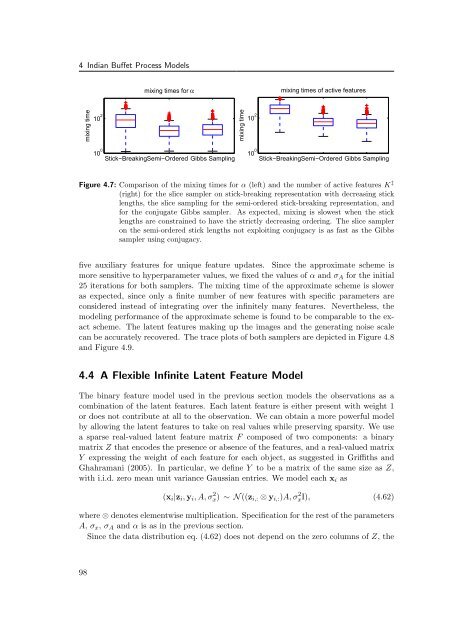
Figure 4.7: Comparison of the mixing times for α (left) and the number of active features K ‡
(right) for the slice sampler on stick-breaking representation with decreasing stick
lengths, the slice sampling for the semi-ordered stick-breaking representation, and
for the conjugate Gibbs sampler. As expected, mixing is slowest when the stick
lengths are constrained to have the strictly decreasing ordering. The slice sampler
on the semi-ordered stick lengths not exploiting conjugacy is as fast as the Gibbs
sampler using conjugacy.
five auxiliary features for unique feature updates. Since the approximate scheme is
more sensitive to hyperparameter values, we fixed the values of α and σA for the initial
25 iterations for both samplers. The mixing time of the approximate scheme is slower
as expected, since only a finite number of new features with specific parameters are
considered instead of integrating over the infinitely many features. Nevertheless, the
modeling performance of the approximate scheme is found to be comparable to the exact
scheme. The latent features making up the images and the generating noise scale
can be accurately recovered. The trace plots of both samplers are depicted in Figure 4.8
and Figure 4.9.
4.4 A Flexible Infinite Latent Feature Model
The binary feature model used in the previous section models the observations as a
combination of the latent features. Each latent feature is either present with weight 1
or does not contribute at all to the observation. We can obtain a more powerful model
by allowing the latent features to take on real values while preserving sparsity. We use
a sparse real-valued latent feature matrix F composed of two components: a binary
matrix Z that encodes the presence or absence of the features, and a real-valued matrix
Y expressing the weight of each feature for each object, as suggested in Griffiths and
Ghahramani (2005). In particular, we define Y to be a matrix of the same size as Z,
with i.i.d. zero mean unit variance Gaussian entries. We model each xi as
(xi|zi, yi, A, σ 2 x) ∼ N ((zi,: ⊗ yi,:)A, σ 2 xI), (4.62)
where ⊗ denotes elementwise multiplication. Specification for the rest of the parameters
A, σx, σA and α is as in the previous section.
Since the data distribution eq. (4.62) does not depend on the zero columns of Z, the
98