Boundary-layer height detection with a ceilometer at a coastal ... - Orbit

More documents

Recommendations

Info

5 Results 5.1 Clouds A simple estimate of cloud cover is made from the ceilometer data. Every time the backscatter signal exceeds 1000/(10 8 m srad), the algorithm indicates either cloud or fog and the time step is noted as a cloud observation. As mentioned in section 3 the ceilometer measurements cover the period from April 2010 to March 2011 with 10 s time resolution. From the analysis of the 10 min data stored in the database, it is seen that 58 % of the time the presence of clouds is detected within the vertical range of 200 – 3000 m. The starting height of 200 m is chosen to avoid mist events that give very high backscatter values at the lowest measuring heights. 2000 ! profile 17/05/2010 Smoothed**profile 19:50 17/05/2010 19:50 2000 2000 smooth /z profile 17/05/2010 19:50 1800 1800 1800 1600 1600 1600 1400 1400 1400 1200 1200 1200 Height [m] 1000 Height [m] 1000 Height [m] 1000 800 800 800 600 600 600 400 400 400 200 200 200 0 0 −500 0 5000 1000 0 1500 5000 10000 Backscatter [1/(10 8 *srad*m)] Backscatter [1/(10 8 srad m)] (a) 0 100 50 0 50 100 Backscatter gradient [1/(10 8 *srad*m 2 )] (b) 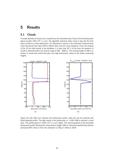Figure 16: Left: Blue line indicates the backscatter profile, while the red line indicates the fitted idealized profile. The high values in the backscatter at ∼1100–1300 m indicate a cloud layer. The profile peaks at 13000/(10 8 m srad). Right: The vertical gradient of the smoothed backscatter profile. Backscatter values peak at height 1200 m. Horizontal dashed lines indicate estimated BLH. Data is from the ceilometer on May 17 2010 at 19:50. 29
Decoupled Clouds Clouds that are not boundary-layer clouds, i.e. those that are decoupled from the ABL or well above it, still influence the BLH detection. As seen in Figure 16 the cloud signal dominates the backscatter profile where the highest signals are ∼ 13000/(10 8 m srad). Both the fitting of the idealized profile seen in Figure 16(a) and the vertical gradient of the smoothed backscatter seen in Figure 16(b) fail to detect the BLH that is seen to be at ∼400 m. The idealized profile method finds the minimized differences by identifying the BLH at the cloud base at ∼1110 m. The vertical gradient method identifies the BLH at the cloud top at ∼1250 m. 17/05/2010 19:50 1600 Zero filter 1600 Linear interpolation 1600 Cloud base filter 1400 1400 1400 1200 1200 1200 1000 1000 1000 Height [m] 800 Height [m] 800 Height [m] 800 600 600 600 400 400 400 200 200 200 0 100 200 Backscatter [1/(10 8 *srad*m)] 0 100 200 Backscatter [1/(10 8 *srad*m)] 0 100 200 Backscatter [1/(10 8 *srad*m)] Figure 17: Plots of three different cloud filtering methods with associated fitting of the idealized profile. Blue lines indicate backscatter profile while red lines indicate idealized profile. Horizontal dotted lines indicate BLH estimates. Data taken from the ceilometer May 17 2010 at 19:50. Filtering decoupled clouds improves the BLH detection significantly. This is seen in Figure 17 showing three different cloud filtering methods (the zero filter, linear interpolation and cloud base filter) and the idealized profile BLH detection method. This figure shows the same backscatter profile as in Figure 16 only with the cloud filtering applied. The cloud signal does not dominate the backscatter profile any longer and the idealized profile now makes a better fit, identifying the BLH right above 400 m. It is seen in Figure 17 that the BLH estimates are independent of the chosen cloud filtering method. This is because in this case the cloud is ∼700 m above the detected ABL. However in conditions with a cloud topped ABL, the chosen cloud filtering method will influence the BLH estimate of all methods. The cloud topped boundary layer In situations with a CTBL, the BLH detection methods often detect the BLH at the top of the cloud. This might not always cause wrong detections, depending on the chosen BLH definition with a cloud topped boundary layer. As mentioned in section 2.7 when a CTBL is 30 DTU Wind Energy Master Thesis M-0039
Page 1 and 2: DTU Wind Energy Master Thesis M-003
Page 3 and 4: Contents 1 Introduction 5 1.1 Thesi
Page 5 and 6: 1.1 Thesis contents The content of
Page 7 and 8: and Batchvarova, 1994; Stull, 1988)
Page 9 and 10: ∂ē ∂t = g w ′ θ v ′ − u
Page 11 and 12: 2.7 Boundary-layer clouds The prese
Page 13 and 14: the square root of the variance. Ro
Page 15 and 16: 3 Site and measurements In this sec
Page 17 and 18: occasionally use the term “radial
Page 19 and 20: Ultrasonic Wind Sensor uSonic-3 Sci
Page 21 and 22: 4 Boundary-layer height detection T
Page 23 and 24: 90/(10 8 m srad), respectively). Fo
Page 25 and 26: 1400 β profile 16/04/2010 11:40 14
Page 27: 24/04/2010 06:20 1000 σ w 1000 ē
Page 31 and 32: 1600 Zero filter 23/07/2010 22:00 N
Page 33 and 34: 5.2 Continuous and average data The
Page 35 and 36: of the error bars during the day. T
Page 37 and 38: also be explained by the shape of t
Page 39 and 40: increases from 19:00-20:00. A resid
Page 41 and 42: 1400 1200 BLH estimations 01/05/201
Page 43 and 44: 5.4 Cold front passage On April 8 2
Page 45 and 46: Wind vectors at 10m height. Metmast
Page 47 and 48: 0.3 The inverse Obukhov length 1/L
Page 49 and 50: Wind vectors at 10m height. Metmast
Page 51 and 52: 0.1 The inverse Obukhov length 1/L
Page 53 and 54: 1400 BLH from minimum TKE 16 June 2
Page 55 and 56: 70 60 Threshold night day Easterly
Page 57 and 58: Threshold Westerly winds Ideal prof
Page 59 and 60: 140 120 Threshold night day Easterl
Page 61 and 62: Threshold Easterly winds Ideal prof
Page 63 and 64: 400 300 Threshold night day Easterl
Page 65 and 66: 5.9 Intra-annual variation The BLH
Page 67 and 68: wind lidar (Sathe et al., 2011). Ho
Page 69 and 70: distributions. It is clear that the
Page 71 and 72: A Appendix Abbreviations ABL Atmosp
Page 73 and 74: References Batchvarova, E., X. Cai,
Page 75: Sinclair, V. A., S. Niemelä, and M

Boundary-layer height detection with a ceilometer at a coastal ... - Orbit

You also want an ePaper? Increase the reach of your titles

Delete template?

Save as template?