Boundary-layer height detection with a ceilometer at a coastal ... - Orbit

observed and the cloud layer and boundary layer are turbulently fully coupled then defining
the BLH at the top of the cloud may be preferable. When working with ceilometer data alone,
it cannot be determined if the two layers are fully coupled and it may be convenient to define
the BLH in another manner than at the cloud top.
1600
Zero filter
23/07/2010 22:00
Nearest−neighbour interpolation
1600
1600
Cloud base filter
1400
1400
1400
1200
1200
1200
1000
1000
1000
Height [m]
800
Height [m]
800
Height [m]
800
600
600
600
400
400
400
200
200
200
0
0 100 200
Backscatter [1/(10 8 *srad*m)]
0
0 100 200
Backscatter [1/(10 8 *srad*m)]
0
0 100 200
Backscatter [1/(10 8 *srad*m)]
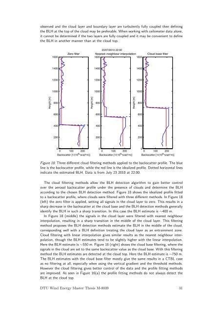
Figure 18: Three different cloud filtering methods applied to the backscatter profile. The blue
line is the backscatter profile, while the red line is the idealized profile. Dotted horizontal lines
indicate the estimated BLH. Data is from July 23 2010 at 22:00.
The cloud filtering methods allow the BLH detection algorithm to gain better control
over the aerosol backscatter profile under the presence of clouds and determine the BLH
according to the chosen BLH detection method. Figure 18 shows the idealized profile fitted
to a backscatter profile, where clouds were filtered with three different methods. In Figure 18
(left) the zero filter is applied, setting all signals in the cloud layer to zero. This results in a
sharp decrease in the backscatter at the cloud base and the BLH detection methods generally
identify the BLH in such a sharp transition. In this case the BLH estimate is ∼400 m.
In Figure 18 (middle) the signals in the cloud layer were filtered with nearest neighbour
interpolation, resulting in a sharp transition in the middle of the cloud layer. This filtering
method proposes the BLH detection methods estimate the BLH in the middle of the cloud,
corresponding well with a BLH definition treating the cloud layer as an entrainment zone.
Cloud filtering with linear interpolation gives similar results as the nearest neighbour interpolation,
though the BLH estimates tend to be slightly higher with the linear interpolation.
Here the BLH estimate is ∼550 m. Figure 18 (right) shows the cloud base filtering, where the
signals in the cloud are set to the same backscatter value as the cloud base. With this filtering
method the BLH estimates are detected at the cloud top. Here the BLH estimate is ∼750 m.
The BLH estimates with the cloud base filter mostly give the same results in a CTBL case
as no filtering at all, especially when using the vertical gradient and the threshold methods.
However the cloud filtering gives better control of the data and the profile fitting methods
are improved. As seen in Figure 16(a) the profile fitting methods do not always detect the
BLH at the cloud top.
DTU Wind Energy Master Thesis M-0039 31