Boundary-layer height detection with a ceilometer at a coastal ... - Orbit

files show a shape that fits well with the exponent idealized profile, i.e increasing backscatter
values from ∼ 100 m down to the surface. The exponent idealized profile method detects the
BLH with the least σ, only differing one meter between the 10 min and 10 s data.
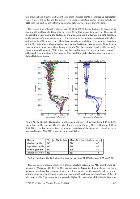
The second time interval is chosen from 09:00 to 09:10 during daytime. In Figure 24 is
shown plots analogous to those seen in Figure 23 for this second time interval. The error of
the signal is greater during the daytime as the ambient sunlight influences the light detection
of the ceilometer’s laser among others. This is seen by the standard deviations both above
and within the ABL being greater than those seen during nighttime. The standard deviation
of the BLH estimates is also noticeably larger during daytime as may be seen in Table 4, with
values up to 6 times larger than during nighttime (for the exponent ideal profile method).
Hennemuth and Lammert (2006) noted that this variability may be caused by single convective
eddies with a time scale of a few minutes. The variability might also be caused by gravity- or
Kelvin-Helmholtz waves.
1000
10 sec. backscatter profiles
1000
10 min. mean backscatter profile
900
900
800
800
700
700
600
600
Height [m]
500
Height [m]
500
400
400
300
300
200
200
100
100
−100 0 100 200 300
−100 0 100 200 300
Backscatter [1/(10 8 *srad*m 2 )]
Backscatter [1/(10 8 *srad*m 2 )]
Figure 24: On the left: Backscatter profiles measured every 10 seconds from 9:00 to 9:10.
Every third profile is shown. On the right: The average of the sixty 10 s profiles from 9:00 to
9:10. With error bars representing the standard deviation of the backscatter signal at every
measured height. The BLH is seen to be around 300 m.
Method BLH [m] 10min data Mean BLH [m] 10s data σ [m]
Idealized profile 343 316 47
Exp. ideal. profile 343 319 45
Vertical gradient 340 326 51
Critical threshold 360 333 46
Table 4: Results of the BLH detection methods on June 21 2010 between 9:00 and 9:10.
The averaging procedure results in a thicker interface between the ABL and the free atmosphere
(Wyngaard, 2010). The 10 s profiles seen in Figure 24 show a sharper, or more
horizontal interfacial layer compared with the 10 min mean. But the variability of the height
of these sharp interfacial layers results in a very smooth and large interfacial layer of the 10
min mean profile. The reason for the generally higher BLH estimates of the 10 min data may
DTU Wind Energy Master Thesis M-0039 37