NUMERICAL SIMULATION OF LOW-SPEED STALL AND ... - IAG

applied to simulate an infinite wing without any tip or
wind tunnel side wall effects. The distance between
the periodic planes was chosen as big as possible
under consideration of limited computational costs to
minimise the error introduced through the forced span
wise periodicity of the flow. The numerical schemes
were the same as applied to URANS. During one time
step of 2.5µs the flow passes the shortest cells in
the wake which, in combination with the isotropically
structured mesh, ensures a low dissipation in the
propagation of the turbulent wake structures.
4. RESULTS
4.1. URANS Simulations
The analysis of the 2d URANS simulations
concentrates on the SST turbulence model because
it is used for the semi-empirical turbulent fluctuation
spectrum model later. The results with the other
eddy-viscosity turbulence models are comparable. In
the simulations the boundary layer flow separates from
the suction side of the airfoil, as expected from the
compared experimental data. The unsteady flow is
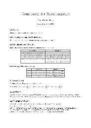
exactly periodic with a very long main cycle of about
11.5 convective time scales (see Figure 2). Over a
big part of this period the separated flow reattaches to
the upper surface of the airfoil and forms a separation
bubble (see Figure 3 a)). Gradually the separation point
is moving upstream and the vortex inside the bubble is
getting stronger. This becomes significant in the rising
lift coefficient during this phase. There is virtually no
large-scale turbulent movement in the wake.
1.6
1.4
c l
1.2
1
0.8
0 5 10 15 20 25 30 35 40
t U c ∞
Figure 2. c l time series of a NACA 0012 airfoil at
16 ◦ angle of attack (URANS SST)
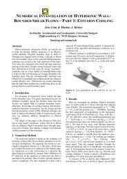
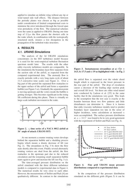
At one moment a counter rotating vortex develops
behind the separation bubble and a shedding process
begins which means a drastic decrease of lift (see
Fig. 2). The streamlines in Fig. 3 b) show the flow
state shortly after this event. Finally several alternately
rotating vortices are shed from the airfoil, the flow
reattaches in the upstream part due to the reduced
circulation and the remaining small separation bubble
starts again to grow and increase the lift (see Fig. 3 c)).
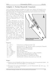
The time-averaged pressure distribution on the
airfoil simulated with the three different turbulence
models is compared to experimental data in Figure 4.
The numerical results lie very close to each other.
However, the measurements of Seifert and Pack [4] are
qualitatively different. In contrast to the simulations
a)
b)
c)
Figure 3. Instantaneous streamlines at a) t U∞ c
=
14.5, b) 17.5 and c) 19 as highlighted with◦in Fig. 2
the airfoil flow is separated over the whole chord
length which is expressed in the lower pressure in
the rear part of the airfoil. The drop of circulation
causes a decrease of the leading edge suction peak
and overall lift level. Yet there are older wind tunnel
tests conducted by Ladson et al. [25] in the same
facility that fit the simulations very good. This leads
to the assumption that the test case is exactly at the
boarder between those two flow patterns and little
disturbances can determine it. Since it is known
that eddy-viscosity turbulence models tend to predict
boundary layer separation too late in the sense of
higher incidence, some calculations at increased α
were accomplished. The surface pressure distribution
at α = 18.5 ◦ was found to be in very good agreement
with the experiment of Seifert and Pack (see Fig. 4).
-6
-5
-4
c
-3
p
-2
-1
0
1
16° Exp. Seifert
16° Exp. Ladson
16° C-grid URANS SAO
16° C-grid URANS SST
16° C-grid URANS RSM
18.5° C-grid URANS SST
0 0.2 0.4 0.6 0.8 1
x/c
Figure 4. Fine grid URANS mean pressure
distributions compared to experimental data
In the comparison of the pressure distribution
simulated on the different grids (Figure 5) it can be
202