NUMERICAL SIMULATION OF LOW-SPEED STALL AND ... - IAG

medium mesh results in Fig. 6) the same characteristics
are expected as with the fine DDES mesh. According
studies also discussing different DES formulations are
to be published by Illi et al. [26].
Another approach to gain information about the
turbulent spectrum is to perform the relatively cheap
URANS and model a turbulence spectrum from the
turbulent quantities calculated by the turbulence model.
This is done for the presented test case in the following
section.
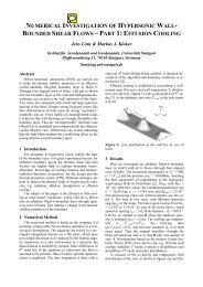
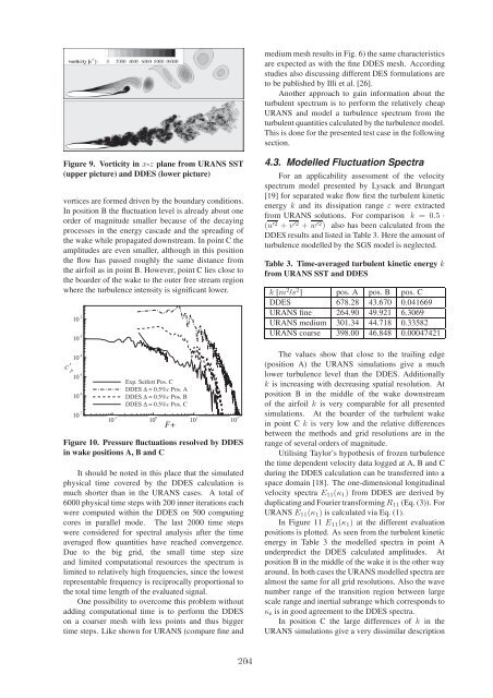
Figure 9. Vorticity in x-z plane from URANS SST
(upper picture) and DDES (lower picture)
vortices are formed driven by the boundary conditions.
In position B the fluctuation level is already about one
order of magnitude smaller because of the decaying
processes in the energy cascade and the spreading of
the wake while propagated downstream. In point C the
amplitudes are even smaller, although in this position
the flow has passed roughly the same distance from
the airfoil as in point B. However, point C lies close to
the boarder of the wake to the outer free stream region
where the turbulence intensity is significant lower.
10 -3
4.3. Modelled Fluctuation Spectra
For an applicability assessment of the velocity
spectrum model presented by Lysack and Brungart
[19] for separated wake flow first the turbulent kinetic
energy k and its dissipation range ε were extracted
from URANS solutions. For comparison k = 0.5 ·
(u ′2 + v ′2 + w ′2 ) also has been calculated from the
DDES results and listed in Table 3. Here the amount of
turbulence modelled by the SGS model is neglected.
Table 3. Time-averaged turbulent kinetic energy k
from URANS SST and DDES
k [m 2 /s 2 ] pos. A pos. B pos. C
DDES 678.28 43.670 0.041669
URANS fine 264.90 49.921 6.3069
URANS medium 301.34 44.718 0.33582
URANS coarse 398.00 46.848 0.00047421
10 -2 Exp. Seifert Pos. C
c’ p
10 -4
10 -5
10 -6
10 -7
DDES ∆ = 0.5%c Pos. A
DDES ∆ = 0.5%c Pos. B
DDES ∆ = 0.5%c Pos. C
10 -1 10 0 10
F+
1 10 2
Figure 10. Pressure fluctuations resolved by DDES
in wake positions A, B and C
It should be noted in this place that the simulated
physical time covered by the DDES calculation is
much shorter than in the URANS cases. A total of
6000 physical time steps with 200 inner iterations each
were computed within the DDES on 500 computing
cores in parallel mode. The last 2000 time steps
were considered for spectral analysis after the time
averaged flow quantities have reached convergence.
Due to the big grid, the small time step size
and limited computational resources the spectrum is
limited to relatively high frequencies, since the lowest
representable frequency is reciprocally proportional to
the total time length of the evaluated signal.
One possibility to overcome this problem without
adding computational time is to perform the DDES
on a coarser mesh with less points and thus bigger
time steps. Like shown for URANS (compare fine and
The values show that close to the trailing edge
(position A) the URANS simulations give a much
lower turbulence level than the DDES. Additionally
k is increasing with decreasing spatial resolution. At
position B in the middle of the wake downstream
of the airfoil k is very comparable for all presented
simulations. At the boarder of the turbulent wake
in point C k is very low and the relative differences
between the methods and grid resolutions are in the
range of several orders of magnitude.
Utilising Taylor’s hypothesis of frozen turbulence
the time dependent velocity data logged at A, B and C
during the DDES calculation can be transferred into a
space domain [18]. The one-dimensional longitudinal
velocity spectra E 11 (κ 1 ) from DDES are derived by
duplicating and Fourier transformingR 11 (Eq. (3)). For
URANS E 11 (κ 1 ) is calculated via Eq. (1).
In Figure 11 E 11 (κ 1 ) at the different evaluation
positions is plotted. As seen from the turbulent kinetic
energy in Table 3 the modelled spectra in point A
underpredict the DDES calculated amplitudes. At
position B in the middle of the wake it is the other way
around. In both cases the URANS modelled spectra are
almost the same for all grid resolutions. Also the wave
number range of the transition region between large
scale range and inertial subrange which corresponds to
κ e is in good agreement to the DDES spectra.
In position C the large differences of k in the
URANS simulations give a very dissimilar description
204