preconditioners for linearized discrete compressible euler equations

European Conference on Computational Fluid Dynamics 

ECCOMAS CFD 2006 

P. Wesseling, E. Oñate and J. Périaux (Eds) 

c○ TU Delft, The Netherlands, 2006 

PRECONDITIONERS FOR LINEARIZED DISCRETE 

COMPRESSIBLE EULER EQUATIONS 

Bernhard Pollul ∗ † 

∗ RWTH Aachen University, IGPM (Institut für Geometrie und Praktische Mathematik) 

Templergraben 55, D-52065 Aachen, Germany 

e-mail: pollul@igpm.rwth-aachen.de 

web page: http://www.igpm.rwth-aachen.de/pollul/ 

† This research was supported by the German Research Foundation 

through the Collaborative Research Centre SFB 401 

Key words: Euler Equations, Krylov Subspace Methods, Point-Block Preconditioners 

Abstract. We consider a Newton-Krylov approach for discretized compressible Euler 

equations. A good preconditioner in the Krylov subspace method is essential for obtaining 

an efficient solver in such an approach. In this paper we compare point-block-Gauss-Seidel, 

point-block-ILU and point-block-SPAI preconditioners. It turns out that the SPAI method 

is not satisfactory for our problem class. The point-block-Gauss-Seidel and point-block- 

ILU preconditioners result in iterative solvers with comparable efficiencies. 

1 INTRODUCTION 

We are interested in iterative methods for solving the large sparse nonlinear systems of 

equations that result from the discretization of stationary compressible Euler equations. 

Related to the discretization it is important to distinguish two approaches. Firstly, a 

direct spatial discretization (using finite differences or finite volume techniques) applied 

to the stationary problem results in a corresponding nonlinear discrete problem. In the 

second approach the stationary solution is characterized as the asymptotic (i.e., time 

tending to infinity) solution of an evolution problem. In such a setting one applies a 

time integration method to the instationary Euler equations. In cases where one has very 

small spatial grid sizes, for example if one uses grids with strong local refinements, an 

implicit time integration method should be used. This then yields a nonlinear system of 

equations in each timestep. Note that for a given spatial grid in the first approach we 

have one discrete nonlinear problem whereas in the second approach we obtain a sequence 

of discrete nonlinear problems. 

For solving such nonlinear systems of equations there are many different approaches. Here 

we mention two popular techniques, namely nonlinear multigrid solvers and Newton- 

Krylov methods. Well-known nonlinear multigrid techniques are the FAS method by 

1

Bernhard Pollul 

Brandt [11], the nonlinear multigrid method by Hackbusch [16] and the algorithm introduced 

by Jameson [20]. It has been shown that a nonlinear multigrid approach can result 

in very efficient solvers, which can even have optimal complexity ([21, 25, 26, 28]). For 

these methods, however, a coarse-to-fine grid hierarchy must be available. The Newton- 

Krylov algorithms do not require this. In these methods one applies a linearization technique 

combined with a preconditioned Krylov subspace algorithm for solving the resulting 

linear problems. One then only needs the system matrix and hence these methods are in 

general much easier to implement than multigrid solvers. Moreover, one can use efficient 

implementations of templates that are available in sparse matrix libraries. Due to these 

attractive properties the Newton-Krylov technique is also often used in practice (cf., for 

example, [27, 29, 30, 31, 32, 42]). 

In this paper we consider the Newton-Krylov approach. A method of this class has been 

implemented in the QUADFLOW package, which is an adaptive multiscale finite volume 

solver for stationary and instationary compressible flow computations. A description 

of this solver is given in [4, 8, 9, 10, 37]. For the linearization we use a standard (approximate) 

Newton method. The resulting linear systems are solved by a preconditioned 

BiCGSTAB method. The main topic of this paper is a systematic comparative study 

of different basic preconditioning techniques. The preconditioners that we consider are 

based on the so-called point-block approach in which all physical unknowns corresponding 

to a grid point or a cell are treated as a block unknown. As preconditioners we use the 

point-block-Gauss-Seidel (PBGS), point-block-ILU (PBILU(0)) and point-block sparse 

approximate inverse (PBSPAI(0)) methods. The main motivation for considering the 

PBSPAI(0) preconditioner is that opposite to the other two preconditioners this method 

allows a trivial parallelization. We do not know of any literature in which for compressible 

flows the SPAI technique is compared with the more classical ILU and Gauss-Seidel 

preconditioners. In our comparative study we consider three test problems. The first 

one is a stationary Euler problem on the unit square with boundary conditions such that 

the problem has a trivial constant solution. For the second test problem we change the 

boundary conditions such that the problem has a solution consisting of three different 

states separated by shocks, that reflect at the upper boundary. In these first two test 

problems we use the Van Leer flux vector-splitting scheme [24] for discretization. We do 

not use an (artificial) time integration method. The third test problem is the stationary 

Euler flow around an NACA0012 airfoil. This standard case is also used for testing the 

QUADFLOW solver in [10]. Discretization is based on the flux-vector splitting method of 

Hänel and Schwane [18] combined with a linear reconstruction technique. For determining 

the stationary solution a variant of the backward Euler scheme (the b2-scheme by Batten 

et. al. [6]) is used. For these three test problems we perform numerical experiments for 

different flow conditions and varying mesh sizes. 

While the PBSPAI(0) preconditioner turns out to unsuitable, the efficiencies of the 

PBGS preconditioner and the PBILU(0) method are comparable. Both depend on the 

ordering of the unknowns [2, 7, 17, 32]. Further improvement of these preconditioners 

2


can be achieved by using numbering techniques. These are well-known for PBILU(0) (e.g. 

[13, 14]). For PBGS we discussed several numbering techniques in [33]. To illustrate the 

improvement due to numbering we present a result for PBGS with a particular numbering 

technique from [33]. 

2 DISCRETE EULER EQUATIONS 

In this section we introduce three test problems that are used for a comparative study 

of different preconditioners. In the first two of these test problems we consider a relatively 

simple model situation with a standard first order flux vector-splitting scheme on 

a uniform grid in 2D. In the third test problem we consider more advanced finite volume 

techniques on locally refined grids as implemented in the QUADFLOW package. 

2.1 Test problem 1: Stationary 2D Euler with constant solution 

In this section we consider a very simple problem which, however, is still of interest for 

the investigation of properties of iterative solvers. We take Ω = [0, 1] 2 and consider the 

stationary Euler equations in differential form: 

⎛ 

∂f(u) 

∂x 

+ ∂g(u) 

∂y 

⎞ 

ρv 1 

= 0 , f(u) := ⎜ρv1 2 + p 

⎟ 

⎝ ρv 1 v 2 

⎠ , 

ρv 1 h tot 

⎛ ⎞ 

ρv 2 

g(u) := ⎜ ρv 1 v 2 

⎝ρv 2 2 + p 

⎟ 

⎠ . (1) 

ρv 2 h tot 

Here u = (ρ, ρv, ρe tot ) T ∈ R 4 is the vector of unknown conserved quantities: ρ denotes 

the density, p the pressure, v = (v 1 , v 2 ) T the velocity vector, e tot the total energy and 

h tot the total enthalpy. The system is closed by the equation of state for a perfect gas 

p = ρ(γ−1)(e tot −1/2|v| 2 ), where γ is the ratio of specific heats, which for air has the value 

γ = 1.4. The boundary conditions (for the primitive variables) are taken such that these 

Euler equations have a constant solution. For the velocity we take v = (v in ) with given 

1 , vin 2 

constants vi in > 0, i = 1, 2, on the inflow boundary Γ in = { (x, y) ∈ ∂Ω | x = 0 or y = 0 }. 

For the density we select a constant value ρ = ρ in > 0 on Γ in . For the pressure we also take 

a constant value p = ¯p > 0 which is prescribed either at the inflow boundary (supersonic 

case) or at outflow boundary ∂Ω \Γ in (subsonic case). The Euler equations (1) then have 

a solution that is constant in the whole domain: v = (v1 in, 

vin 2 ), ρ = ρin , p = ¯p. 

For the discretization of this problem we use a uniform mesh Ω h = { (ih, jh) | 0 ≤ i, j ≤ 

n }, with nh = 1, and apply a basic upwinding method, namely the Van Leer flux vectorsplitting 

scheme [24]. The discretization of (physical and numerical) boundary conditions 

is based on compatibility relations (section 19.1.2 in [19]). In each grid point we then 

have four discrete unknowns, corresponding to the four conserved quantities. We use a 

lexicographic ordering of the grid points with numbering 1, 2, . . ., (n+1) 2 =: N. The four 

unknowns at grid point i are denoted by U i = (u i,1 , u i,2 , u i,3 , u i,4 ) T and all unknowns are 

collected in the vector U = (U i ) 1≤i≤N . The discretization yields a nonlinear system of 

3


equations 

1 

❛ 

❛ 

❛ 

I 

❛❛❛ III 

❛ 

II ❛❛❛❛ 

0 ✑ ✑✑✑✑✑✑✑✑ ❛ ❛ ❛ 

0 1 2 3 4 

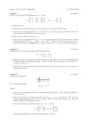
Figure 1: Three different states separated by shocks 

F : R 4N → R 4N , F(U) = 0 . (2) 

The continuous constant solution (restricted to the grid) solves the discrete problem and 

thus the solution of the nonlinear discrete problem in 2 is known a-priori. This solution 

is denoted by U ∗ . For the Jacobian DF(U) of F(U) explicit formulas can be derived. In 

section 4 we investigate the behavior of different preconditioners when applied to a linear 

system of the form 

DF(U ∗ )x = b . (3) 

Note that the matrix DF(U ∗ ) has a regular block structure 

DF(U ∗ ) = blockmatrix(A i,j ) 0≤i,j≤N 

with A i,j ∈ R 4×4 for all i, j. We call this a point-block structure. Furthermore, A i,j ≠ 0 

can occur only if i = j or i and j correspond to neighboring grid points. 

2.2 Test problem 2: Stationary 2D Euler with shock reflection 

We consider a two-dimensional stationary Euler problem presented in example 5.3.3 

in [23]. The domain is Ω = [0, 4] × [0, 1] and for the boundary conditions we take ρ = 

1.4, v 1 = 2.9, v 2 = 0, p = 1.0 at the left boundary (x = 0), outflow boundary conditions 

at the right boundary (x = 4), ρ = 2.47, v 1 = 2.59, v 2 = 0.54, p = 2.27 at the lower 

boundary (y = 0) and reflecting boundary conditions at the upper boundary (y = 1). 

With these boundary conditions the problem has a stationary solution consisting of three 

different states separated by shocks, that reflect at the upper boundary, cf. figure 1. For 

the discretization of this problem we apply the same method as in test problem 1. This 

results in a nonlinear system of equations as in 2, but now the discrete solution, denoted by 

U ∗ , is not known a-priori. In a Newton type of method applied to this nonlinear problem 

one has to solve linear systems with matrix DF(Ũ), Ũ ≈ U∗ . Therefore we investigate 

iterative solvers applied to DF(U ∗ )x = b. The discrete solution U ∗ is computed up to 

machine accuracy using some time integration method. Note that the Jacobian matrix 

DF(U ∗ ) has a similar point-block structure as the Jacobian matrix in test problem 1. 

4


2.3 Test problem 3: Stationary flow around NACA0012 airfoil 

The third problem is a standard test case for inviscid compressible flow solvers. We 

consider the inviscid, transonic stationary flow around the NACA0012 airfoil (cf. [22]). 

The discretization is based on the conservative formulation of the Euler equations. For 

an arbitrary control volume V ⊂ Ω ⊂ R 2 one has equations of the form 

∫ 

∂u 

∂t 

∮∂V 

dV + F c (u)n dS = 0 . (4) 

V 

Here n is the outward unit normal on ∂V , u the vector of unknown conserved quantities 

and the convective flux is given by 

⎛ 

ρv 

⎞ 

F c (u) = ⎝ ρv ◦ v + pI ⎠ . (5) 

ρh tot v 

The symbol ◦ denotes the dyadic product. As above the system is closed by the equation 

of state for a perfect gas. The discretization of these equations is based on cell centered 

finite volume schemes on an unstructured mesh as implemented in QUADFLOW and 

explained in [10]. For the present test problem the flux-vector splitting due to Hänel and 

Schwane [18] is applied. Note that this is a variant of the Van Leer flux-vector splitting 

method that is used in the previous two test problems. In our experiments the Van 

Leer method and the Hänel-Schwane method give similar results both with respect to 

discretization quality and with respect to the performance of iterative solvers. A linear 

reconstruction technique is used to obtain second order accuracy in regions where the 

solution is smooth. This is combined with the Venkatakrishnan limiter [41]. Although we 

are interested in the stationary solution of this problem the time derivative is not skipped. 

This time derivative is discretized by a time integration method which then results in a 

numerical method for approximating the stationary solution. To allow a fast convergence 

towards the stationary solution one wants to use large timesteps and thus an implicit 

time discretization method is preferred. This approach then results in a nonlinear system 

of equations in each timestep. Here we use the b2-scheme by Batten et. al. [6] for time 

integration. Per timestep one inexact Newton iteration is applied. In this inexact Newton 

method an approximate Jacobian is used, in which the linear reconstruction technique is 

neglected and the Jacobian of the first order Hänel-Schwane discretization is approximated 

by one-sided difference operators (as in [40]). These Jacobian matrices have the structure 

DF(U) = diag ( |V i | ) ∂R HS (U) + 

∆t ∂U 

, (6) 

where |V i | is the volume of a control volume V i , ∆t the (local) timestep and R HS (U) 

the residual vector corresponding to the Hänel-Schwane fluxes. Details are given in [10]. 

5


Note that in general a smaller timestep will improve the conditioning of the approximate 

Jacobian in (6). 

We start with an initial coarse grid and an initial CFL number C MIN , which determines 

the size of the timestep. After each timestep in the time integration the CFL number (and 

thus the timestep) is increased by a constant factor until an a-priori fixed upper bound 

C MAX is reached. Time integration is continued until a tolerance criterion for the residual 

is satisfied. Then a (local) grid refinement is performed and the procedure starts again 

with an initial CFL number equal to C MIN . The indicator for the local grid refinement 

is based on a multiscale analysis using wavelets [10]. In every timestep one approximate 

Newton iteration is performed. The resulting linear equation is solved with a user defined 

accuracy for the relative residual. The approximate Jacobian has a point-block structure 

as in the first two test problems: DF(U) = blockmatrix(A i,j ) 0≤i,j≤N with A i,j ∈ R 4×4 for 

all i, j and A i,j ≠ 0 only if i = j or i and j correspond to neighboring cells. 

3 POINT-BLOCK-PRECONDITIONERS 

In the three test problems described above we have to solve a large sparse linear system. 

The matrices in these systems are sparse and have a point-block structure in which the 

blocks correspond to the 4 unknowns in each of the N grid points (finite differences) or 

N cells (finite volume). Thus we have linear systems of the form 

Ax = b , A = blockmatrix(A i,j ) 1≤i,j≤N , A i,j ∈ R 4×4 . (7) 

For the type of applications that we consider these problems are often solved by using 

a preconditioned Krylov-subspace method. In our numerical experiments we use the 

BiCGSTAB method. In the following subsections we describe basic point-block iterative 

methods that are used as preconditioners in the iterative solver. For the right handside 

we use a block representation b = (b 1 , . . ., b N ) T , b i ∈ R 4 , that corresponds to the block 

structure of A. The same is done for the iterands x k that approximate the solution of 

the linear system in (7). 

For the description of the preconditioners the nonzero pattern P(A) corresponding to 

the point-blocks in the matrix A is important: 

3.1 Point-block-Gauss-Seidel method 

P(A) = { (i, j) | A i,j ≠ 0 } . (8) 

The point-block-Gauss-Seidel method (PBGS) is the standard block Gauss-Seidel 

method applied to (7). Let x 0 be a given starting vector. Then for k ≥ 0 the iterand 

x k+1 = (x k+1 

1 , . . .,x k+1 )T should satisfy 

N 

A i,i x k+1 

i 

∑i−1 

= b i − 

j=1 

A i,j x k+1 

j 

− 

N∑ 

j=i+1 

6 

A i,j x k j , i = 1, . . ., N . (9)


This method is well-defined if the 4 × 4 linear systems in 9 are uniquely solvable, i.e., 

if the diagonal blocks A i,i are nonsingular. In our applications this was always satisfied. 

This elementary method is very easy to implement and needs no additional storage. The 

algorithm is available in the PETSc library [3]. A Convergence analysis of this method 

for the 1D stationary Euler problem is presented in [34]. 

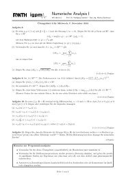
3.2 Point-block-ILU(0) method 

We consider the following point-block version of the standard point ILU(0) algorithm: 

for k = 1, 2, . . ., N − 1 

D := A −1 

k,k ; 

for i = k + 1, k + 2, . . ., N 

if (i, k) ∈ P(A) 

E := A i,k D ; A i,k := E ; 

for j = k + 1, k + 2, . . ., N 

if (i, j) ∈ P(A) and (k, j) ∈ P(A) 

A i,j := A i,j − EA k,j ; 

end if 

end j 

end if 

end i 

end k 

Figure 2: Point-block-ILU(0) algorithm 

This algorithm is denoted by PBILU(0). Note that as for the PBGS method the diagonal 

blocks A k,k are assumed to be nonsingular. For this preconditioner a preprocessing 

phase is needed in which the incomplete factorization is computed. Furthermore additional 

storage similar to the storage requirements for the matrix A is needed. 

As for point ILU methods one can consider variants of this algorithm in which a larger 

pattern as P(A) is used and thus more fill-in is allowed (cf. for example, ILU(p), [35]). 

Both the PBILU(0) algorithm and such variants are available in the PETSc library. 

7


3.3 Block sparse approximate inverse 

In the SPAI method [15, 38] an approximate inverse M of the matrix A is constructed 

by minimizing the Frobenius norm ‖AM − I‖ F with a prescribed sparsity pattern of the 

matrix M. In the point-block version of this approach (cf. [5]), denoted by PBSPAI(0), 

we take a block representation M = blockmatrix(M i,j ) 1≤i,j≤N , M i,j ∈ R 4×4 , and the set 

of admissible approximate inverses is given by 

M := {M ∈ R 4N×4N | P(M) ⊆ P(A) } . (10) 

A sparse approximate inverse M is determined by minimization over this admissible set 

‖AM − I‖ F = min ‖A ˜M − I‖ F . 

˜M∈M 

The choice for the Frobenius norm allows a splitting of this minimization problem. Let 

˜M j = blockmatrix( ˜M i,j ) 1≤i≤N ∈ R 4N×4 be the j-th block column of the matrix ˜M and I j 

the corresponding block column of I. Let ˜m j,k and e j,k , k = 1, . . .,4, be the k-th columns 

of the matrix ˜M j and I j , respectively. As a result of 

N 

‖A ˜M − I‖ 2 F = ∑ 

‖A ˜M j − I j ‖ 2 F = 

j=1 

N∑ 4∑ 

‖A ˜m j,k − e j,k ‖ 2 2 (11) 

j=1 k=1 

the minimization problem can be split into 4N decoupled least squares problems: 

min 

˜m j,k 

‖A ˜m j,k − e j,k ‖ 2 , j = 1, . . ., N, k = 1, . . .,4. (12) 

The vector ˜m j,k has the block representation ˜m j,k = (m 1 , . . .,m N ) T with m l ∈ R 4 and 

m l = 0 if (l, j) /∈ P(A). Hence for fixed (j, k) and with e j,k =: (e 1 , . . .,e N ) T , e l ∈ R 4 , we 

have 

N∑ ∗ 

‖A ˜m j,k − e j,k ‖ 2 2 = ‖A i,l m l − e l ‖ 2 2 

i,l=1 

where in the double sum ∑ ∗ 

only pairs (i, l) occur with (i, l) ∈ P(A) and (l, j) ∈ P(A). 

Thus the minimization problem for the column ˜m j,k in (12) is a low dimensional least 

squares problem that can be solved by standard methods. Due to (11) these least squares 

problems for the different columns of the matrix M can be solved in parallel. Moreover 

the application of the PBSPAI(0) preconditioner requires a sparse matrix-vector product 

computation which is also has a high parallelization potential. As for the PBILU(0) 

preconditioner a preprocessing phase is needed in which the PBSPAI(0) preconditioner 

M is computed. Additional storage similar to the storage requirements for the matrix A 

is needed. 

8


In the literature a row-variant of SPAI is also used. This method is based on the 

minimization problem 

‖MA − I‖ F = min ‖ ˜MA − I‖ F . 

˜M∈M 

A row-wise decoupling leads to a very similar method as the one described above. Here 

we denote this algorithm by PBSPAI row (0). 

As for the ILU preconditioner these SPAI preconditioners have variants in which additional 

fill-in is allowed, cf. [5, 15]. Besides as a preconditioner the SPAI method can also be 

used as a smoother in multigrid solvers (cf. [12, 39]). 

4 NUMERICAL EXPERIMENTS 

In this section we present results of numerical experiments. Our goal is to illustrate 

and to compare the behavior of the different preconditioners presented above for a few 

test problems. The first two test problems (described in section 2.1 and 2.2) are Jacobian 

systems that result from the Van Leer flux vector-splitting discretization on a uniform 

mesh with mesh size h, cf. (3). These Jacobians are evaluated at the discrete solution 

U ∗ . In the first test problem this solution is a trivial one (namely, constant), whereas in 

the second test problem we have a reflecting shock. In the third test case we have linear 

systems with matrices as in (6) that arise in the solver used in the QUADFLOW package. 

In all experiments below we use a left preconditioned BiCGSTAB method. For the 

first two test problems, the discretization routines, methods for the construction of the 

Jacobian matrices and the preconditioners (PBGS, PBILU(0) and PBSPAI(0)) are implemented 

in MATLAB. We use the BiCGSTAB method available in MATLAB. For the 

third test problem the approximate Jacobian matrices as in (6) are computed in QUAD- 

FLOW. For the preconditioned BiCGSTAB method and the PBGS, PBILU(p), p = 0, 1, 2, 

preconditioners we use routines from the PETSc library [3]. 

To measure the quality of the preconditioners we present the number of iterations that 

is needed to satisfy a certain tolerance criterion. To allow a fair comparison of the different 

preconditioners we briefly comment on the arithmetic work needed for the construction 

of the preconditioners and the arithmetic costs of one application of the preconditioners. 

As unit of arithmetic work we take the costs of one matrix-vector multiplication with the 

matrix A (=: 1 matvec). For the PBGS method we have no construction costs. The arithmetic 

work per application of PBGS is about 0.7 matvec. Note that both in PBILU(0) 

and PBSPAI(0) the nonzero block-pattern is not larger that of the matrix A (e.g., for 

PBSPAI(0), P(M) ⊆ P(A) in (10)). However, in a nonzero block of the matrix A certain 

entries can be zero, whereas in the preconditioner the corresponding entries may be 

nonzero. For example, in the shock reflection test problem, about one fourth of the entries 

in the nonzero blocks are zero, whereas in the PBILU(0) and PBSPAI(0) preconditioners 

for this problem almost all entries in the nonzero blocks are nonzero. In our experiments 

the costs for constructing the PBILU(0) preconditioner are between 2 and 4 matvecs. We 

typically need 1.2-1.6 matvecs per application of PBILU(0). The costs for constructing 

9


the PBSPAI(0) preconditioner are much higher (note, however, the high parallelization 

potential). Typical values (depending on P(A)) in our experiments are 20-50 matvecs. 

In the application of this preconditioner no 4 × 4 subproblems have to be solved and due 

to this the arithmetic work is somewhat less as for the PBILU(0) preconditioner. We 

typically need 1.2-1.5 matvecs per application of the PBSPAI(0) preconditioner. Summarizing, 

if we only consider the costs per application of the preconditioners than the 

PBILU(0) method is about twice as expensive as the PBGS method and the PBSPAI(0) 

preconditioner is slightly less expensive than the PBILU(0) method. 

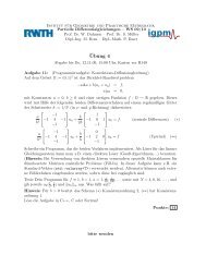
4.1 Test problem 1: Stationary 2D Euler with constant solution 

We consider the discretized stationary Euler equations described in test problem 1 

with mesh size h = 0.02. We vary the Mach number in x-direction, which is denoted 

by M x : 0.05 ≤ M x ≤ 1.25. For the Mach number in y-direction, denoted by M y , we 

take M y = 3M 2 x. The linear system in (3) is solved with the preconditioned BiCGSTAB 

method, with starting vector zero. The iteration is stopped if the relative residual (2- 

norm) is below 1E-6. Results are presented in Figure 3. As a result of the downwind 

numbering the upper block-diagonal part of the Jacobian is zero in the supersonic case 

(M x > 1) and thus both the PBILU(0) method and PBGS are exact solvers. The PB- 

SPAI(0) preconditioner does not have this property, due to the fact that M is a sparse 

Figure 3: Test problem 1, iteration count 

10


approximation of A −1 , which is a dense point-block lower triangular matrix. For M x < 1 

with PBGS preconditioning we need about 1 to 4 times as much iterations as with 

PBILU(0) preconditioning. Both preconditioners show a clear tendency, namely that 

the convergence becomes faster if M x is increased. For M x < 1 the PBSPAI(0) preconditioners 

shows an undesirable very irregular behavior. There are peaks in the iteration 

counts close to M x = 2 3 (hence, M y = 1) and M x = 1. Applying BiCGSTAB without 

preconditioning we observe divergence for most M x values and if the method converges 

then its rate of convergence is extremely low. 

4.2 Test problem 2: Stationary 2D Euler with shock reflection 

We consider the discretized stationary Euler equations with a shock reflection as described 

in section 2.2 on grids with different mesh sizes h x = h y = 2 −k , k = 3, . . ., 7. The 

discrete solution U ∗ is determined with high accuracy using a damped Newton method. 

As in section 4.1 we use the preconditioned BiCGSTAB method to solve a linear system 

with matrix DF(U ∗ ) until the relative residual is below 1E-6. The number of iterations 

that is needed is shown in table 1. The symbol † denotes that the method did not converge 

within 2000 iterations. Both for the PBGS and the PBILU(0) preconditioner we observe 

the expected h −1 

y behavior in the iteration counts. With PBGS preconditioning one needs 

about 1.5 to 2 times as much iterations as with PBILU(0) preconditioning. Again the 

performance of the PBSPAI(0) preconditioner is very poor. 

mesh size h y 

1 

8 

1 

16 

1 

32 

1 

64 

1 

128 

PBGS 15 26 51 108 232 

PBILU(0) 10 17 30 59 109 

PBSPAI(0) 183 † † † † 

PBSPAI row (0) 193 † † † † 

Table 1: Test problem 2, iteration count 

4.3 Test Problem 3: Stationary flow around NACA0012 airfoil 

We consider two standard NACA0012 airfoil test cases ([22] test cases 3 and 1; the 

other three reference test cases for this airfoil yield similar results) as described in test 

problem 3. Test case A corresponds to the flow parameters M ∞ = 0.95, α = 0 ◦ (also used 

in [10]) and test case B corresponds to the parameters M ∞ = 0.8, α = 1.25 ◦ . Related 

to the discretization we recall some facts from [10]. The far-field boundary is located 

about 20 chord lengths from the airfoil. Standard characteristic boundary conditions are 

applied at the far-field. Computations are initialized on a structured grid consisting of 

11


4 blocks with 10 × 10 cells each. Adaptation of the grid was performed each time the 

density residual has decreased two orders of magnitude. On the finest level the iteration 

is stopped when the density residual is reduced by a factor of 10 4 . Grid refinement and 

coarsening are controlled by a multiscale wavelet technique. For test case A this results 

in a sequence of 14 (locally refined) grids. In table 2 we show the number of cells in 

each of these grids. We note that on the finer grids a change (refinement/coarsening) to 

Grid 1 2 3 4 5 6 7 

# cells 400 1,600 4,264 7,006 11,827 15,634 21,841 

Grid 8 9 10 11 12 13 14 

# cells 25,870 28,627 30,547 31,828 33,067 33,955 34,552 

Table 2: Test case A, sequence of grids 

the next grid does not necessarily imply a smaller finest mesh size. It may happen that 

only certain coarse cells are refined to obtain a better shock resolution. For a discussion 

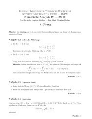
of this adaptivity issue we refer to [10]. In figure 4 the final grid (34,552 cells) and the 

corresponding Mach number distribution is shown. 

The flow pattern downstream of the trailing edge has a complex shock configuration. 

Two oblique shocks are formed at the trailing edge. The supersonic region behind these 

oblique shocks is closed by a further normal shock. 

On each grid an implicit time integration is applied (cf. section 2.3). Currently the 

choice of the timestep is based on an ad hoc strategy. Starting with a CFL number 

equal to 1 the timestep is increased based on the rule CFL new = 1.1 CFL old . A maximum 

value of 1000 is allowed. Per timestep one inexact Newton iteration is applied. The 

linear systems with the approximate Jacobians (cf. section 2.3) are solved by a preconditioned 

BiCGSTAB method until the relative residual is smaller than 1E-2. Because the 

PBSPAI(0) preconditioners have shown a very poor behavior already for the relatively 

simple problems in section 4.1 and section 4.2 we decided not to use the PBSPAI(0) 

preconditioner in this test problem. An interface between QUADFLOW and the PETSc 

library [3] has been implemented. This makes the BiCGSTAB method and PBILU(0) preconditioner 

available. Recently also a PBGS routine has become available. The PETSc 

library offers many other iterative solvers and preconditioners. Here, besides the PBGS 

and PBILU(0) preconditioners we also consider block variants of ILU that allow more 

fill-in, namely the PBILU(1) and PBILU(2) methods. 

The arithmetic work in the QUADFLOW solver is dominated by the linear solves on 

the finest grids. We present results only for the two finest grids. The corresponding 

number of preconditioned BiCGSTAB iterations for each timestep on these two grids 

is given in figure 5. Note that different preconditioners may lead to (slightly) different 

numbers of timesteps. On grid 13 we have about 110 timesteps and then a change to 

grid 14 takes place. In these 110 timesteps on grid 13 the iteration count shows a clear 

12


Figure 4: Test case A. Left figure: computational grid. Right figure: Mach distribution, M min = 0.0, 

M max = 1.45, ∆M = 0.05 

increasing trend. This is due to the increase of the CFL number. After the change to grid 

14 one starts with CFL = 1 and a similar behaviour occurs again. 

test case A B 

Grid 13 14 10 11 

PBGS 15.3 20.2 2.85 32.0 

PBILU(0) 6.92 8.82 1.33 11.2 

PBILU(1) 4.49 4.65 1.04 6.87 

PBILU(2) 3.52 3.81 1.04 5.78 

Table 3: Test cases A and B, average iteration count 

13


Figure 5: Test case A, iteration count 

In test case B the adaptivity strategy results in 11 grids. In table 3 for both test cases 

we show the averaged number of preconditioned BiCGSTAB iterations for the two finest 

grids, where the average is taken over the time steps per grid. 

Note that with PBGS we need 2.1-2.8 times more iterations as with PBILU(0) and with 

PBILU(2) we need about 2 times less iterations as with PBILU(0). Taking the arithmetic 

work per iteration into account we conclude that PBGS and PBILU(0) have comparable 

efficiency, whereas the PBILU(p), p = 1, 2, preconditioners are (much) less efficient. 

To illustrate the dependence of the rate of convergence on the mesh size we consider, for 

test case A, a sequence of uniformly refined grids, cf. table 4. On every grid we continue 

the time integration until the density residual has decreased two orders of magnitude. 

Iteration counts are shown in table 5. 

From these results we see that due to the mass matrix coming from the (artificial) time 

integration the average iteration count increases much slower as h −1 . The total number of 

Grid 1 2 3 4 5 

# cells 400 1,600 6,400 25,600 102,400 

Table 4: sequence of uniformely refined grids 

14


Grid 1 2 3 4 5 

PBGS 5.8 9.2 13.3 18.2 21.7 

PBILU(0) 1.9 2.4 2.9 4.3 4.5 

PBILU(1) 1.6 1.7 1.9 2.7 2.9 

PBILU(2) 1.0 1.4 1.8 1.9 2.0 

Grid 1 2 3 4 5 

PBGS 947 1806 3739 9030 19212 

PBILU(0) 301 462 806 2121 4025 

PBILU(1) 250 335 547 1324 2562 

PBILU(2) 161 274 510 940 1783 

Table 5: Test case A. Average iteration count (above) and sum over all time steps per grid (below). 

iterations, however, shows a clear h −1 behaviour as in the model problem in section 4.2. 

The large total number of iterations needed on fine grids (table 5, right) is caused by the 

many timesteps that are needed. A significant improvement of efficiency may come from 

a better strategy for the timestep control. 

Remark Incomplete LU-factorization and Gauss-Seidel techniques are popular preconditioners 

that are used in solvers in the numerical simulation of compressible flows [1, 2, 32, 

36]. Both preconditioners depend on the ordering of the cells (grid-points) [2, 7, 17, 32]. 

In combination with PBILU the reverse Cuthill-McKee ordering algorithm [13, 14] is often 

used. This ordering yields a matrix with a “small” bandwidth. 

In [33] we investigated ordering algorithms for the PBGS preconditioner and introduced 

a ‘weighted reduced graph numbering’ (WRG) which turned out to give good results 

compared to other renumbering algorithms. This WRG numbering is particularly effective 

for supersonic flows. Therefore a result for M ∞ = 1.2, α = 0 ◦ (cf. [22]), denoted by C, 

is presented in table 6, too. The columns QN show the average iteration count when 

applying PBGS with the numbering induced by the solver QUADFLOW. The iteration 

count can be reduced by 8.9% - 51.5% when coupling PBGS with WRG numbering. 

The cost for computing the renumbering is negligible because the permutation is only 

computed once on every level of adaptation. When using a (point-block) random numtest 

case A B C 

numbering QN WRG QN WRG QN WRG 

PBGS 20.2 18.4 32.0 23.0 20.6 10.0 

Table 6: Test cases A,B and C, average iteration count on finest adaptation level 

15


bering, the PBGS-preconditioned BiCGSTAB method does not converge in most cases. 

With WRG numbering, though, even with large CFL-numbers (e.g. 1000, 5000) the linear 

solver converges in most cases if we use PBGS. The WRG algorithm is black-box 

and significantly improves the robustness and efficiency of the point-block Gauss-Seidel 

preconditioner. For further explanation and properties of this and other renumbering 

algorithms we refer to [33]. 

5 CONCLUSIONS 

We summarize the main conclusions. Already for our relatively simple model problems 

the PBSPAI(0) method turns out to be a poor preconditioner. This method should not 

be used in a Newton-Krylov method for solving compressible Euler equations. Both for 

model problems and a realistic application (QUADFLOW solver for NACA0012 airfoil) 

the efficiencies of the PBGS preconditioner and the PBILU(0) method are comparable. 

For our applications the PBILU(1) and PBILU(2) preconditioners are less efficient than 

the PBILU(0) preconditioner. To achieve a robust preconditioner PBILU(0) and PBGS 

can be coupled with a suitable ordering algorithm. 

Acknowledgement 

The experiments in section 4.3 are carried ot using the QUADFLOW solver developed 

in the Collaborative Research Center SFB 401 [37]. The authors acknowledge the fruitful 

collaboration with several members of the QUADFLOW research group. 

REFERENCES 

[1] K. Ajmani, W.-F. Ng and M. Liou, Preconditioned Conjugate Gradient Methods for 

the Navier-Stokes Equations, J. Comp. Phys. 110 68–81 (1994). 

[2] E. F. D’Azevedo, P.A. Forsyth and W.-P. Tang, Ordering Methods for Preconditioned 

Conjugate Gradient Methods Applied to Unstructured Grid Problems, SIAM 

J. Matrix Anal. Appl. 13(3) 944–961 (1992) 

[3] S. Balay, K. Buschelman, W. D. Gropp, D. Kaushik, M. Knepley, L. C. McInnes. B. 

F. Smith and H. Zhang, PETSc, http://www-fp.mcs.anl.gov/petsc/ (2001). 

[4] J. Ballmann (editor), Flow Modulation and Fluid-Structure-Interaction at Airplane 

Wings, Numerical Notes on Fluid Mechanics 84, Springer (2003). 

[5] S. T. Barnard and M. J. Grote, A Block Version of the SPAI Preconditioner, in Proc. 

9th SIAM Conf. On Parallel Process. for Sci. Comp. (1999). 

[6] P. Batten, M. A. Leschziner and U.C. Goldberg, Average-State Jacobians and Implicit 

Methods for Compressible Viscours and Turbulent Flows, J. Comp. Phys. 137, 

38–78 (1997). 

16


[7] Bey, J. Wittum, Downwind numbering: robust multigrid for convection-diffusion 

problems, App. Num. Math. 23 177–192 (1997). 

[8] K.H. Brakhage and S. Müller, Algebraic-hyperbolic Grid Generation with Precise 

Control of Intersection of Angles, Int. J. Numer. Meth. Fluids. 33, 89–123 (2000). 

[9] F. Bramkamp, B. Gottschlich-Müller, M. Hesse, Ph. Lamby, S. Müller, J. Ballmann, 

K.-H. Brakhage, W. Dahmen, H-adaptive Multiscale Schemes for the Compressible 

Navier-Stokes Equations: Polyhedral Discretization, Data Compression and Mesh 

Generation, in [4], 125–204 (2001). 

[10] F. Bramkamp, Ph. Lamby and S. Mller, An adaptive multiscale finite volume solver 

for unsteady and steady state flow comput., J. Comp. Physics, 197/2 460–490 (2004). 

[11] A. Brandt, Multi-level Adaptive Solutions to Boundary Value Problems, Math. 

Comp. 31, 333–390 (1977). 

[12] O. Bröker, M.J. Grote, C. Mayer, A. Reusken, Robust Parallel Smoothing for Multigrid 

via Sparse Approximate Inverses, SIAM J. Sci. Comput. 23 1396–1417 (2001). 

[13] E. Cuthill, Several strategies for reducing the band width of matrices. Sparse Matrices 

and Their Appl., D. J. Rose and R. A. Willoughby, eds., New York, 157–166 (1997). 

[14] E. Cuthill, J. McKee, Reducing the bandwidth of sparse symmetric matrices. in: 

Proc. ACM Nat. Conf., New York, 157–172 (1969). 

[15] M.J. Grote and T. Huckle, Parallel Preconditioning with Sparse Approximate Inverses, 

SIAM J. Scient. Comput. 18(3) (1997). 

[16] W. Hackbusch, Multi-grid Methods and Applications, Springer (1985). 

[17] W. Hackbusch, On the Feedback Vertex Set for a Planar Graph, Computing 58 

129–155, (1997). 

[18] D. Hänel and F. Schwane, An Implicit Flux-Vector Splitting Scheme for the Computation 

of Viscous Hypersonic Flow, AIAA paper 0274 (1989). 

[19] C. Hirsch, Numerical computation of internal and external flows: computational 

methods for inviscid and viscous flows, 2, Wiley (1988). 

[20] A. Jameson, Solution of the Euler Equations for Two-Dimensional Transonic Flow 

by a Multigrid Method, Appl. Math. Comp. 13 327–356 (1983). 

[21] A. Jameson, D.A. Caughey, How Many Steps are Required to Solve the Euler Equations 

of Steady, Compressible Flow: in search of a Fast Solution Algorithm, AIAA 

paper 2673 (2001). 

17


[22] D. J. Jones, Reference Test Cases and Contributors, Test Cases For Inviscid Flow 

Field Methods. AGARD Advisory Report 211(5) (1986). 

[23] D. Kröner, Numerical schemes for conservation laws, Wiley (1997). 

[24] B. van Leer, Flux Vector Splitting for the Euler Equations. In: Proceedings of the 

8th International Conference on Numerical Methods in Fluid Dynamics (E. Krause, 

ed.). Lecture Notes in Physics 170 507–512. Springer, Berlin (1982). 

[25] B. van Leer and D. Darmofal, Steady Euler Solutions in O(N) Operations, Multigrid 

Methods (E. Dick, K. Riemslagh and J. Vierendeels, editors) VI 24–33 (1999). 

[26] I. Lepot, P. Geuzaine, F. Meers, J.-A. Essers and J.-M. Vaassen, Analysis of Several 

Multigrid Implicit Algorithms for the Solution of the Euler Equations on Unstructured 

Meshes, Multigrid Meth. VI 157–163 (1999). 

[27] H. Luo, J. Baum and R. Loehner, A Fast, Matrix-free Implicit Method for Compressible 

Flows on Unstructured Grids, J. Comp. Phys. 146 664–690 (1998). 

[28] D.J. Mavripilis and V. Venkatakrishnan, Implicit method for the Computation of 

Unsteady Flows on Unstructured Grids, J. Comp. Phys., 127 380–397 (1996). 

[29] P.R. McHugh and D.A. Knoll, Comparison of Standard and Matrix-Free Implementations 

of Several Newton-Krylov Solvers, AIAA J. 32 394–400 (1994). 

[30] A. Meister, Comparison of different Krylov Subspace Methods Embedded in an Implicit 

Finite Volume Scheme for the Computation of Viscous and Inviscid Flow Fields 

on Unstructured Grids, J. of Comp. Phys. 140 311–345 (1998). 

[31] A. Meister, Th. Sonar, Finite-Volume Schemes for Compressible Fluid Flow. Surv. 

Math. Ind. 8 1–36 (1998). 

[32] A. Meister, C. Vömel, Efficient Preconditioning of Linear Systems Arising from the 

Discretization of Hyperbolic Conservation Laws, Adv. Comp. Math. 14 49–73 (2001). 

[33] B. Pollul and A. Reusken, Numbering Techniques for Preconditioners in Iterative 

Solvers for Compressible Flows, submitted to Int. J. Numer. Meth. Fluids. (2006). 

[34] A. Reusken, Convergence analysis of the Gauss–Seidel Preconditioner for Discretized 

One Dimensional Euler Equations, SIAM J. Numer. Anal. 41 1388–1405 (2003). 

[35] Y. Saad, Iterative methods for sparse linear systems, PWS Publishing Company, 

Boston (1996). 

18


[36] Y. Saad, Preconditioned Krylov Subspace Methods for CFD Applications, in:, Solution 

techniques for Large-Scale CFD-Problems, ed. W.G. Habashi, Wiley, 139–158 

(1995). 

[37] SFB 401, Collaborative Research Center, Modulation of flow and fluidstructure 

interaction at airplane wings, RWTH Aachen University of Technology, 

http://www.lufmech.rwth-aachen.de/sfb401/kufa-e.html 

[38] W.-P. Tang, Toward an Effective Approximate Inverse Preconditioner, SIAM J. Matrix 

Anal. Appl. 20 970–986, (1999). 

[39] W.-P. Tang and W. L. Wan, Sparse Approximate Inverse Smoother for Multigrid, 

SIAM J. Matrix Anal. Appl. 21 1236–1252 (2000). 

[40] K.J. Vanden and P. D. Orkwis, Comparison of Numerical and Analytical Jacobians, 

AIAA J. 34(6) 1125–1129 (1996). 

[41] V. Venkatakrishnan, V., Convergence to Steady State Solutions of the Euler Equations 

on Unstructured Grids with Limiters, J. Comp. Phys. 118 120–130 (1995). 

[42] V. Venkatakrishnan, Implicit schemes and Parallel Computing in Unstructured Grid 

CFD, ICASE-report 28 (1995). 

19

preconditioners for linearized discrete compressible euler equations

Create successful ePaper yourself

Delete template?

Save as template?