preconditioners for linearized discrete compressible euler equations

Bernhard Pollul
equations
1
❛
❛
❛
I
❛❛❛ III
❛
II ❛❛❛❛
0 ✑ ✑✑✑✑✑✑✑✑ ❛ ❛ ❛
0 1 2 3 4
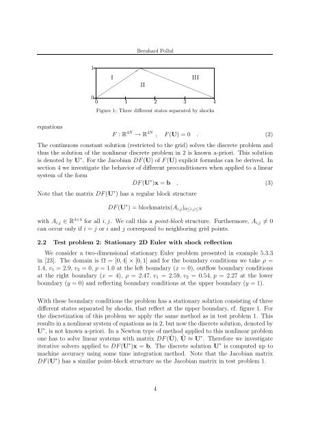
Figure 1: Three different states separated by shocks
F : R 4N → R 4N , F(U) = 0 . (2)
The continuous constant solution (restricted to the grid) solves the discrete problem and
thus the solution of the nonlinear discrete problem in 2 is known a-priori. This solution
is denoted by U ∗ . For the Jacobian DF(U) of F(U) explicit formulas can be derived. In
section 4 we investigate the behavior of different preconditioners when applied to a linear
system of the form
DF(U ∗ )x = b . (3)
Note that the matrix DF(U ∗ ) has a regular block structure
DF(U ∗ ) = blockmatrix(A i,j ) 0≤i,j≤N
with A i,j ∈ R 4×4 for all i, j. We call this a point-block structure. Furthermore, A i,j ≠ 0
can occur only if i = j or i and j correspond to neighboring grid points.
2.2 Test problem 2: Stationary 2D Euler with shock reflection
We consider a two-dimensional stationary Euler problem presented in example 5.3.3
in [23]. The domain is Ω = [0, 4] × [0, 1] and for the boundary conditions we take ρ =
1.4, v 1 = 2.9, v 2 = 0, p = 1.0 at the left boundary (x = 0), outflow boundary conditions
at the right boundary (x = 4), ρ = 2.47, v 1 = 2.59, v 2 = 0.54, p = 2.27 at the lower
boundary (y = 0) and reflecting boundary conditions at the upper boundary (y = 1).
With these boundary conditions the problem has a stationary solution consisting of three
different states separated by shocks, that reflect at the upper boundary, cf. figure 1. For
the discretization of this problem we apply the same method as in test problem 1. This
results in a nonlinear system of equations as in 2, but now the discrete solution, denoted by
U ∗ , is not known a-priori. In a Newton type of method applied to this nonlinear problem
one has to solve linear systems with matrix DF(Ũ), Ũ ≈ U∗ . Therefore we investigate
iterative solvers applied to DF(U ∗ )x = b. The discrete solution U ∗ is computed up to
machine accuracy using some time integration method. Note that the Jacobian matrix
DF(U ∗ ) has a similar point-block structure as the Jacobian matrix in test problem 1.
4