preconditioners for linearized discrete compressible euler equations

Bernhard Pollul
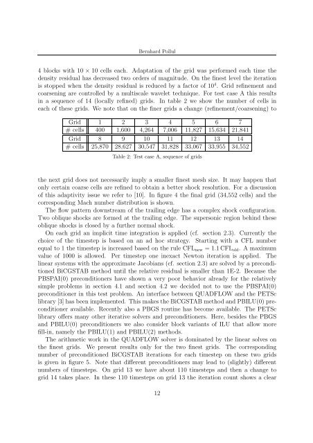
4 blocks with 10 × 10 cells each. Adaptation of the grid was performed each time the
density residual has decreased two orders of magnitude. On the finest level the iteration
is stopped when the density residual is reduced by a factor of 10 4 . Grid refinement and
coarsening are controlled by a multiscale wavelet technique. For test case A this results
in a sequence of 14 (locally refined) grids. In table 2 we show the number of cells in
each of these grids. We note that on the finer grids a change (refinement/coarsening) to
Grid 1 2 3 4 5 6 7
# cells 400 1,600 4,264 7,006 11,827 15,634 21,841
Grid 8 9 10 11 12 13 14
# cells 25,870 28,627 30,547 31,828 33,067 33,955 34,552
Table 2: Test case A, sequence of grids
the next grid does not necessarily imply a smaller finest mesh size. It may happen that
only certain coarse cells are refined to obtain a better shock resolution. For a discussion
of this adaptivity issue we refer to [10]. In figure 4 the final grid (34,552 cells) and the
corresponding Mach number distribution is shown.
The flow pattern downstream of the trailing edge has a complex shock configuration.
Two oblique shocks are formed at the trailing edge. The supersonic region behind these
oblique shocks is closed by a further normal shock.
On each grid an implicit time integration is applied (cf. section 2.3). Currently the
choice of the timestep is based on an ad hoc strategy. Starting with a CFL number
equal to 1 the timestep is increased based on the rule CFL new = 1.1 CFL old . A maximum
value of 1000 is allowed. Per timestep one inexact Newton iteration is applied. The
linear systems with the approximate Jacobians (cf. section 2.3) are solved by a preconditioned
BiCGSTAB method until the relative residual is smaller than 1E-2. Because the
PBSPAI(0) preconditioners have shown a very poor behavior already for the relatively
simple problems in section 4.1 and section 4.2 we decided not to use the PBSPAI(0)
preconditioner in this test problem. An interface between QUADFLOW and the PETSc
library [3] has been implemented. This makes the BiCGSTAB method and PBILU(0) preconditioner
available. Recently also a PBGS routine has become available. The PETSc
library offers many other iterative solvers and preconditioners. Here, besides the PBGS
and PBILU(0) preconditioners we also consider block variants of ILU that allow more
fill-in, namely the PBILU(1) and PBILU(2) methods.
The arithmetic work in the QUADFLOW solver is dominated by the linear solves on
the finest grids. We present results only for the two finest grids. The corresponding
number of preconditioned BiCGSTAB iterations for each timestep on these two grids
is given in figure 5. Note that different preconditioners may lead to (slightly) different
numbers of timesteps. On grid 13 we have about 110 timesteps and then a change to
grid 14 takes place. In these 110 timesteps on grid 13 the iteration count shows a clear
12