Cloud Statistics from Calipso Lidar Data for the ... - espace-tum.de

Chapter 5. Cloud free statistics 48
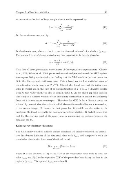
estimates ˆα in the limit of large sample sizes n and is expressed by:
for the continuous case, and by:
ˆα = 1 + n[
ˆα ⋍ 1 + n[
n∑
i=1
ln x i
x min
] −1 (19)
n∑ x i
ln
x min − 1/2 ]−1 (20)
i=1
for the discrete case, where x i , i = 1...n are the observed values of x for which x i ≥ x min .
The standard error of the estimated power law exponent ˆα, is thereby given by:
σ = ˆα − 1 √ n
+ = O(1/n). (21)
Note that all hated parameters are estimates of the respective true parameters. [Clauset
et al., 2009, White et al., 2008] performed several analyses and tested the MLE against
least-square fitting routines with the finding that the MLE result in the best power law
fit in the discrete and continuous case. This is based on the low statistical error of
the estimator, which decays as O(n 1/2 ). Clauset also found out that the initial x min
value is crucial and in the case of an underestimation of x < x min ˆα deviates quickly
from its true value which can also be seen in Table 8. As the cloud gap data used for
this study is a discrete version of the probability distribution it cannot be accurately
fitted with its continuous counterpart. Therefore the MLE fit for a discrete power law
is found by numerical optimization in which the continuous distribution is summed up
to the nearest integer. To ensure the best power law fit possible, an alternative to the
maximum likelihood method is the Kolmogorov-Smirnov statistic. It finds the x min that
best fits the starting point of the power law, by minimizing the distance between the
data and the fit.
Kolmogorov-Smirnov distance:
The Kolmogorov-Smirnov statistic simply calculates the distance between the cumulative
distribution function of the estimated data with ˆx min and compares it with the
cumulative distribution function of the fitted model.
D = max
x≥x min
|M(x) − P (x)| (22)
where D is the distance, M(x) is the CDF of the observation data with at least one
value x min and P (x) is the respective CDF of the power law best fitting the data in the
region x ≥ x min . The optimal ˆx min minimizes D.