Sensors and Methods for Mobile Robot Positioning

CHAPTER 2
HEADING SENSORS
Heading sensors are of particular importance to mobile robot positioning because they can help
compensate for the foremost weakness of odometry: in an odometry-based positioning method, any
small momentary orientation error will cause a constantly growing lateral position error. For this
reason it would be of great benefit if orientation errors could be detected and corrected immediately.
In this chapter we discuss gyroscopes and compasses, the two most widely employed sensors for
determining the heading of a mobile robot (besides, of course, odometry). Gyroscopes can be
classified into two broad categories: (a) mechanical gyroscopes and (b) optical gyroscopes.
2.1 Mechanical Gyroscopes
The mechanical gyroscope, a well-known and reliable rotation sensor based on the inertial properties
of a rapidly spinning rotor, has been around since the early 1800s. The first known gyroscope was
built in 1810 by G.C. Bohnenberger of Germany. In 1852, the French physicist Leon Foucault
showed that a gyroscope could detect the rotation of the earth [Carter, 1966]. In the following
sections we discuss the principle of operation of various gyroscopes.
Anyone who has ever ridden a bicycle has experienced (perhaps unknowingly) an interesting
characteristic of the mechanical gyroscope known as gyroscopic precession. If the rider leans the
bike over to the left around its own horizontal axis, the front wheel responds by turning left around
the vertical axis. The effect is much more noticeable if the wheel is removed from the bike, and held
by both ends of its axle while rapidly spinning. If the person holding the wheel attempts to yaw it left
or right about the vertical axis, a surprisingly violent reaction will be felt as the axle instead twists
about the horizontal roll axis. This is due to the angular momentum associated with a spinning
flywheel, which displaces the applied force by 90 degrees in the direction of spin. The rate of
precession 6 is proportional to the applied torque T [Fraden, 1993]:
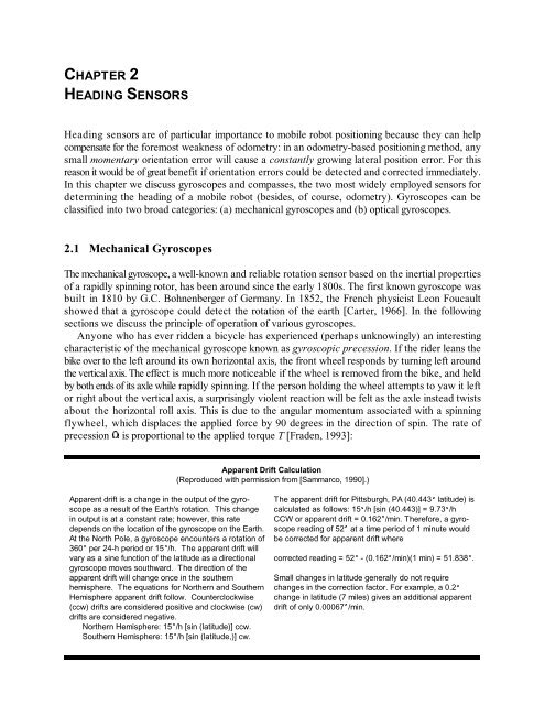
Apparent Drift Calculation
(Reproduced with permission from [Sammarco, 1990].)
Apparent drift is a change in the output of the gyroscope
as a result of the Earth's rotation. This change
in output is at a constant rate; however, this rate
depends on the location of the gyroscope on the Earth.
At the North Pole, a gyroscope encounters a rotation of
360( per 24-h period or 15(/h. The apparent drift will
vary as a sine function of the latitude as a directional
gyroscope moves southward. The direction of the
apparent drift will change once in the southern
hemisphere. The equations for Northern and Southern
Hemisphere apparent drift follow. Counterclockwise
(ccw) drifts are considered positive and clockwise (cw)
drifts are considered negative.
Northern Hemisphere: 15(/h [sin (latitude)] ccw.
Southern Hemisphere: 15(/h [sin (latitude,)] cw.
The apparent drift for Pittsburgh, PA (40.443( latitude) is
calculated as follows: 15(/h [sin (40.443)] = 9.73(/h
CCW or apparent drift = 0.162(/min. Therefore, a gyroscope
reading of 52( at a time period of 1 minute would
be corrected for apparent drift where
corrected reading = 52( - (0.162(/min)(1 min) = 51.838(.
Small changes in latitude generally do not require
changes in the correction factor. For example, a 0.2(
change in latitude (7 miles) gives an additional apparent
drift of only 0.00067(/min.