Empirical Evaluation of Hybrid Defaultable Bond Pricing ... - risklab

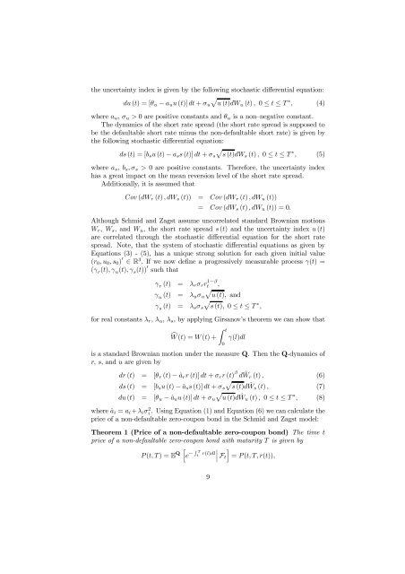
the uncertainty index is given by the following stochastic differential equation:
du (t) =[θ u − a u u (t)] dt + σ u
p
u (t)dWu (t) , 0 ≤ t ≤ T ∗ , (4)
where a u , σ u > 0 are positive constants and θ u is a non—negative constant.
The dynamics of the short rate spread (the short rate spread is supposed to
be the defaultable short rate minus the non-defaultable short rate) is given by
the following stochastic differential equation:
ds (t) =[b s u (t) − a s s (t)] dt + σ s
p
s (t)dWs (t) , 0 ≤ t ≤ T ∗ , (5)
where a s ,b s , σ s > 0 are positive constants. Therefore, the uncertainty index
has a great impact on the mean reversion level of the short rate spread.
Additionally, it is assumed that
Cov(dW r (t) ,dW s (t)) = Cov (dW r (t) ,dW u (t))
= Cov (dW s (t) ,dW u (t)) = 0.
Although Schmid and Zagst assume uncorrelated standard Brownian motions
W r , W s , and W u , the short rate spread s (t) and the uncertainty index u (t)
are correlated through the stochastic differential equation for the short rate
spread. Note, that the system of stochastic differential equations as given by
Equations (3) - (5), has a unique strong solution for each given initial value
(r 0 ,u 0 ,s 0 ) 0 ∈ R 3 . If we now deÞne a progressively measurable process γ(t) =
(γ r (t), γ u (t), γ s (t)) 0 such that
γ r (t) = λ r σ r r 1−β
t ,
p
γ u (t) = λ u σ u u (t), and
p
γ s (t) = λ s σ s s (t), 0 ≤ t ≤ T ∗ ,
for real constants λ r , λ u , λ s , by applying Girsanov’s theorem we can show that
cW (t) =W (t)+
Z t
0
γ(l)dl
is a standard Brownian motion under the measure Q. Then the Q-dynamics of
r, s, and u are given by
dr (t) = [θ r (t) − â r r (t)] dt + σ r r (t) β dŴ r (t) , (6)
p
ds (t) = [b s u (t) − â s s (t)] dt + σ s s (t)dŴs (t) , (7)
p
du (t) = [θ u − â u u (t)] dt + σ u u (t)d Ŵ u (t) , 0 ≤ t ≤ T ∗ , (8)
where â i = a i +λ i σ 2 i . Using Equation (1) and Equation (6) we can calculate the
price of a non-defaultable zero-coupon bond in the Schmid and Zagst model:
Theorem 1 (Price of a non-defaultable zero-coupon bond) The time t
price of a non-defaultable zero-coupon bond with maturity T is given by
P (t, T )=E Q h e − R T
t r(l)dl¯¯¯ Ft
i
= P (t, T, r(t)),
9