Empirical Evaluation of Hybrid Defaultable Bond Pricing ... - risklab

More documents

Recommendations

Info

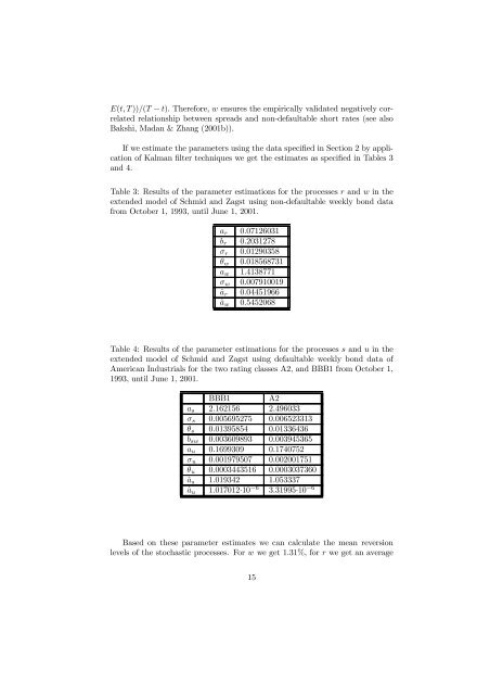
E(t, T ))/(T − t). Therefore, w ensures the empirically validated negatively correlated relationship between spreads and non-defaultable short rates (see also Bakshi, Madan & Zhang (2001b)). If we estimate the parameters using the data speciÞed in Section 2 by application of Kalman Þlter techniques we get the estimates as speciÞed in Tables 3 and 4. Table 3: Results of the parameter estimations for the processes r and w in the extended model of Schmid and Zagst using non-defaultable weekly bond data from October 1, 1993, until June 1, 2001. a r 0.07126031 b r 0.2031278 σ r 0.01290358 θ w 0.018568731 a w 1.4138771 σ w 0.007910019 â r 0.04451966 â w 0.5452068 Table 4: Results of the parameter estimations for the processes s and u in the extended model of Schmid and Zagst using defaultable weekly bond data of American Industrials for the two rating classes A2, and BBB1 from October 1, 1993, until June 1, 2001. BBB1 A2 a s 2.162156 2.496033 σ s 0.005695275 0.006523313 θ s 0.01395854 0.01336436 b sw 0.003609893 0.003945365 a u 0.1699309 0.1740752 σ u 0.001979507 0.002001751 θ u 0.0003443516 0.0003037360 â s 1.019342 1.053337 â u 1.017012·10 −6 3.31995·10 −6 Based on these parameter estimates we can calculate the mean reversion levels of the stochastic processes. For w we get 1.31%, for r we get an average 15
mean reversion level of 5.21%. Thesevaluesarequiteintuitiveastheaverage observed GDP growth rate is around 1.37% and the average observed 3−month rate is approximately 5.12%. For rating categories BBB1 and A2 the mean reversion levels of u are 20 bp, 17 bp, and for s 74 bp, 60 bp, respectively. These numbers are rather intuitive as the average 3−month spreads for rating categories BBB1 and A2 approximately equal 76 bp and 59 bp, respectively, i.e. decrease for ratings of higher quality. 5 The Model of Bakshi, Madan and Zhang In the model of Bakshi et al. (2001a) uncertainty is modeled with a threedimensional standard Brownian motion W = (W r ,W w ,W u ) 0 on the Þltered probability space (Ω, F, F, P). The dynamics of the non-defaultable short rate are described by a two-factor model dr(t) = (w(t) − a r r(t)) dt + σ r q1 − ρ 2 r,wdW r (t)+σ r ρ r,w dW w (t), (22) dw(t) = (θ w − a w w(t)) dt + σ w dW w (t), (23) where a r , a w , σ r ,andσ w , are positive constants, θ w ≥ 0 and |ρ r,w | < 1. The mean reversion level of the short rate r is dependent on w. w is assumed to be unobservable. The short rate spread is modeled according to where u is given by du(t) =(θ u − a u u(t)) dt + σ u ds(t) =(Λ r − 1)dr(t)+Λ u du(t), (24) ρ r,u q 1 − ρ 2 r,w dW r (t)+σ u s 1 − ρ2 r,u 1 − ρ 2 dW u (t). r,w (25) a u and σ u are positive constants, θ u ≥ 0, andρ 2 r,u < 1 − ρ 2 r,w. Therefore, the short rate spread is driven by a factor describing the general state of the economy and a Þrm speciÞc component. Bakshi et al. (2001b) use for u Þrm speciÞc data like stock prices. Note that the system of stochastic differential equations as given by Equations (22) - (25) has a unique strong solution for each given initial value (r 0 ,w 0 ,s 0 ,u 0 ) 0 ∈ R 4 . If we now deÞne a progressively measurable process γ(t) =(γ r (t), γ w (t), γ u (t)) 0 such that γ w (t) = λ w σ w w(t), γ r (t) = λ r σ r r(t) − ρ r,w γ u (t) = λ u σ u u(t) − r 1 − q γ w (t), 1 − ρ 2 r,w ρ r,u √ 1−ρ 2 r,w ρ2 r,u 1−ρ 2 r,w γ r (t) =λ u σ u u(t) − ρ r,u q γ r (t) 1 − ρ 2 r,w − ρ 2 r,u 16
Page 1 and 2: working paper Empirical Evaluation
Page 3 and 4: using a compound options approach a
Page 5 and 6: Þrst introduced by Cathcart & El-J
Page 7 and 8: We assume that there exists a measu
Page 9 and 10: 2,5 2 1,5 1 0,5 1 Year 3 Years 5 Ye
Page 11 and 12: where with ( 1 A(t,T )−B(t,T )r P
Page 13 and 14: a r , b r , σ r , a w , σ w , a u
Page 15: with B(t, T ) = 1 ³ −âr(T 1 −
Page 19 and 20: where P d (t, T, r, w, u) =e Ad (t,
Page 21 and 22: 6 Comparison of the Model Performan
Page 23 and 24: Table 10: Average R 2 values (out
Page 25 and 26: D(0,T)/T*mr% US Industrials A2 US I
Page 27 and 28: 0,8% 0,7% 0,6% US Industrials BBB1
Page 29 and 30: Schmid, Zagst 2000 Schmid, Zagst 20
Page 31 and 32: Hull, J. & White, A. (1990). Pricin
Page 33 and 34: A DeÞnition of v (t, T ) v (t, T )
Page 35 and 36: solution: B(t, T ) = e −âr(T −
Page 37 and 38: D Results of Regression Analyses Ta
Page 39 and 40: Table 17: Test of out—of-sample e

Empirical Evaluation of Hybrid Defaultable Bond Pricing ... - risklab

Create successful ePaper yourself

Delete template?

Save as template?