Ferromagnetic (Ga,Mn)As Layers and ... - OPUS Würzburg

5.2. Magnetic Characterization 77
8 7 .5 0
8 7 .0 0
8 6 .5 0
8 6 .0 0
8 5 .5 0
φ
8 5 .0 0
Ω
8 4 .5 0
4 4 .7 0
4 4 .6 0
4 4 .5 0
φ
4 4 .4 0
4 4 .3 0
-3 0 0 -2 0 0 -1 0 0 0 1 0 0 2 0 0 3 0 0
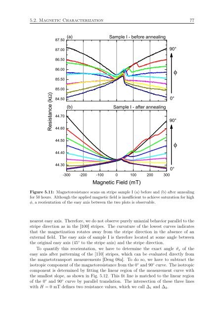
Figure 5.11: Magnetoresistance scans on stripe sample I (a) before and (b) after annealing
for 50 hours. Although the applied magnetic field is insufficient to achieve saturation for high
φ, a reorientation of the easy axis between the two plots is observable.
nearest easy axis. Therefore, we do not observe purely uniaxial behavior parallel to the
stripe direction as in the [100] stripes. The curvature of the lowest curves indicates
that the magnetization rotates away from the stripe direction in the absence of an
external field. The easy axis of sample I is therefore located at some angle between
the original easy axis (45 ◦ to the stripe axis) and the stripe direction.
To quantify this reorientation, we have to determine the exact angle ϑ x of the
easy axis after patterning of the [1¯10] stripes, which can be evaluated directly from
the magnetotransport measurements [Deng 08a]. To do so, we have to subtract the
isotropic component of the magnetoresistance from the 0 ◦ and 90 ◦ curve. The isotropic
component is determined by fitting the linear region of the measurement curve with
the smallest slope, as shown in Fig. 5.12. This fit line is matched to the linear region
of the 0 ◦ and 90 ◦ curve by parallel translation. The intersection of these three lines
with H = 0 mT defines two resistance values, which we call ∆ 1 and ∆ 2 .