Optical Coatings

Fundamental Optics
Material Properties Optical Specifications Gaussian Beam Optics
Paraxial Lens Formulas
PARAXIAL FORMULAS FOR LENSES IN AIR
The following formulas are based on the behavior of paraxial
rays, which are always very close and nearly parallel to the optical
axis. In this region, lens surfaces are always very nearly normal to
the optical axis, and hence all angles of incidence and refraction
are small. As a result, the sines of the angles of incidence and
refraction are small (as used in Snell’s law) and can be approximated
by the angles themselves (measured in radians).
The paraxial formulas do not include effects of spherical
aberration experienced by a marginal ray — a ray passing through
the lens near its edge or margin. All effective focal length values (f)
tabulated in this catalog are paraxial values which correspond to the
paraxial formulas.
The following paraxial formulas are valid for both thick and
thin lenses unless otherwise noted. The refractive index of the lens
glass, n, is the ratio of the speed of light in vacuum to the speed of
light in the lens glass. All other variables are defined in figure 1.33.
Focal Length
1
⎛ 1 1 ⎞ (n 41)
= (n 41)
4 +
f
⎜
⎝ r r
⎟
⎠ n
t c
rr
where n is the refractive index, t c is the center thickness, and the
sign convention previously given for the radii r 1 and r 2 applies. For
thin lenses, t c ≅ 0, and for plano lenses either r 1 or r 2 is infinite. In
either case the second term of the above equation vanishes, and we
are left with the familiar Lens Maker’s formula
1
f
⎛
= (n 41)
⎜ 4
⎝
2
1 1 ⎞
⎟
r1 r2⎠
(1.35)
(1.34)
1 2
1 2
s>0
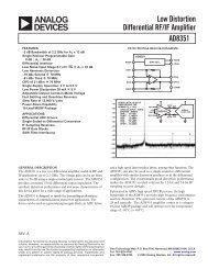
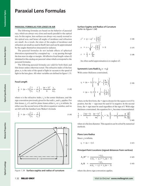
Surface Sagitta and Radius of Curvature
(refer to figure 1.34)
2 2 ⎛ d ⎞
r = (r 4s) + ⎜ ⎟
⎝ 2⎠
2 ⎛ d ⎞
s = r 4 r 4⎜
⎟
⎝ 2⎠
r
1
=
f
2
= s 2 + d .
8s
2
2
> 0
An often useful approximation is to neglect s/2.
Symmetric Lens Radii (r 2 = 5r 1 )
With center thickness constrained,
⎡
⎤
ft
2 c
r 1 = (n 4 1)
⎢ ⎛ ⎞
f ± f 4
⎥
⎢ ⎜
n
⎟
⎝ ⎠
⎥
⎣⎢
⎦⎥
⎡
⎤
tc
= (n 4 1) f
⎢ ⎛ ⎞
1 + 14
⎥
⎢ ⎜
⎝ nf
⎟
⎠
⎥
⎣⎢
⎦⎥
2 (n41)
(n41)
4
r nr
1
2
⎡ ⎧⎪
⎛ f ⎞ ⎫⎪
⎤
⎢t + 2r ⎨14
cos ⎜arcsin ⎝ 2r
⎟ ⎬⎥
⎩⎪
1
⎣
⎢
⎠ ⎭⎪ ⎦
⎥
(1.40)
2 c 1
1
(1.36)
(1.37)
(1.38)
(1.39)
where, in the first form, the + sign is chosen for the square root if f is
positive, but the 4 sign must be used if f is negative. In the second
form, the + sign must be used regardless of the sign of f. With edge
thickness constrained, the equation for r 1 becomes transcendental:
where Ω is the lens diameter. This equation can be solved by numerical
methods.
Plano Lens Radius
Since r 2 is infinite,
r>0
d
2
r 1 = (n 4 1) f.
Principal-Point Locations (signed distances from vertices)
(1.41)
Optical Coatings
(r4s)
Figure 1.34 Surface sagitta and radius of curvature
A H ′′ =
2
AH =
1
4rt
2 c
n (r 4 r ) + t (n 4 1)
2 1 c
4rt
1 c
n (r 4 r ) + t (n 4 1)
2 1 c
where the above sign convention applies.
(1.42)
(1.43)
1.32 1 Visit Us OnLine! www.mellesgriot.com