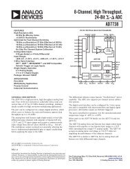
Fundamental Optics Material Properties <strong>Optical</strong> Specifications Gaussian Beam Optics Imaging Properties of Lens Systems THE OPTICAL INVARIANT To understand the importance of the numerical aperture, consider its relation to magnification. Referring to figure 1.6, f NA (object side) = sin v = 2s f NA " (image side) = sin v ′′ = 2s ′′ which can be rearranged to show and f = 2s sinv f = 2s ′′ sinv′′ leading to s′′ s = sin v sinv′′ = NA . NA" Since s ′′ is simply the magnification of the system, s we arrive at m = NA . NA" (1.10) (1.11) (1.12) (1.13) (1.14) (1.15) The magnification of the system is therefore equal to the ratio of the numerical apertures on the object and image sides of the system. This powerful and useful result is completely independent of the specifics of the optical system, and it can often be used to determine the optimum lens diameter in situations involving aperture constraints. When a lens or optical system is used to create an image of a source, it is natural to assume that, by increasing the diameter (f) of the lens, we will be able to collect more light and thereby produce a brighter image. However, because of the relationship between magnification and numerical aperture, there can be a theoretical limit beyond which increasing the diameter has no effect on lightcollection efficiency or image brightness. Since the numerical aperture of a ray is given by f/2s, once a focal length and magnification have been selected, the value of NA sets the value of f. Thus, if one is dealing with a system in which the numerical aperture is constrained on either the object or image side, increasing the lens diameter beyond this value will increase system size and cost but will not improve performance (i.e., throughput or image brightness). This concept is sometimes referred to as the optical invariant. Example: System with Fixed Input NA Two very common applications of simple optics involve coupling light into an optical fiber or into the entrance slit of a monochromator. Although these problems appear to be quite different, they both have the same limitation — they have a fixed numerical aperture. For monochromators, this limit is usually expressed in terms of the f-number. In addition to the fixed numerical aperture, they both have a fixed entrance pupil (image) size. Suppose it is necessary, using a singlet lens from this catalog, to couple the output of an incandescent bulb with a filament 1 mm in diameter into an optical fiber as shown in figure 1.7. Assume that the fiber has a core diameter of 100 mm and a numerical aperture of 0.25, and that the design requires that the total distance from the source to the fiber be 110 mm. Which lenses are appropriate? By definition, the magnification must be 0.1. Letting s + s″ total 110 mm (using the thin-lens approximation), we can use equation 1.3, f = m (s + s ′′ ) (m + 1) 2 to determine that the focal length is 9.1 mm. To determine the conjugate distances, s and s″, we utilize equation 1.6, s (m + 1) = s + s ′′, and find that s = 100 mm and s″ = 10 mm. We can now use the relationship NA = Ω/2s or NA″ = Ω/2s″ to derive Ω, the optimum clear aperture (effective diameter) of the lens. With an image numerical aperture of 0.25 and an image distance (s″) of 10 mm, f 0.25 = 20 f = 5 mm. Accomplishing this imaging task with a single lens therefore requires an optic with a 9.1-mm focal length and a 5-mm diameter. Using a larger diameter lens will not result in any greater system throughput because of the limited input numerical aperture of the optical fiber. The singlet lenses in this catalog that meet these criteria are 01 LPX 003, which is plano-convex, and 01 LDX 003 and 01 LDX 005, which are biconvex. <strong>Optical</strong> <strong>Coatings</strong> SAMPLE CALCULATION To understand how to use this relationship between magnification and numerical aperture, consider the following example. Making some simple calculations has reduced our choice of lenses to just three. Chapter 2, Gaussian Beam Optics, discusses how to make a final choice of lenses based on various performance criteria. 1.6 1 Visit Us OnLine! www.mellesgriot.com
Figure 1.6 Figure 1.7 f f 2 object side magnification = h" = 0.1 = 0.1X h 1.0 filament h = 1 mm v s Numerical aperture and magnification s + s" = 110 mm f NA = = 0.025 2s s = 100 mm optical system f = 9.1 mm f = 5 mm f NA" = = 0.25 2s" fiber core h" = 0.1 mm s" = 10 mm <strong>Optical</strong> system geometry for focusing the output of an incandescent bulb into an optical fiber s″ v″ image side Fundamental Optics Gaussian Beam Optics <strong>Optical</strong> Specifications Material Properties <strong>Optical</strong> <strong>Coatings</strong> Visit Us Online! www.mellesgriot.com 1 1.7