Chapter 14 - Bootstrap Methods and Permutation Tests - WH Freeman
Chapter 14 - Bootstrap Methods and Permutation Tests - WH Freeman
Chapter 14 - Bootstrap Methods and Permutation Tests - WH Freeman

Create successful ePaper yourself
Turn your PDF publications into a flip-book with our unique Google optimized e-Paper software.
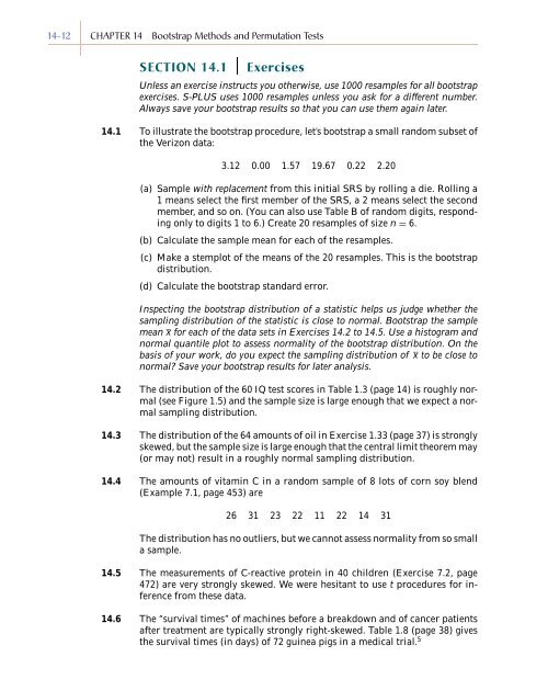
<strong>14</strong>-12 CHAPTER <strong>14</strong> <strong>Bootstrap</strong> <strong>Methods</strong> <strong>and</strong> <strong>Permutation</strong> <strong>Tests</strong><br />
SECTION <strong>14</strong>.1<br />
Exercises<br />
Unless an exercise instructs you otherwise, use 1000 resamples for all bootstrap<br />
exercises. S-PLUS uses 1000 resamples unless you ask for a different number.<br />
Always save your bootstrap results so that you can use them again later.<br />
<strong>14</strong>.1 To illustrate the bootstrap procedure, let’s bootstrap a small r<strong>and</strong>om subset of<br />
the Verizon data:<br />
3.12 0.00 1.57 19.67 0.22 2.20<br />
(a) Sample with replacement from this initial SRS by rolling a die. Rolling a<br />
1 means select the first member of the SRS, a 2 means select the second<br />
member, <strong>and</strong> so on. (You can also use Table B of r<strong>and</strong>om digits, responding<br />
only to digits 1 to 6.) Create 20 resamples of size n = 6.<br />
(b) Calculate the sample mean for each of the resamples.<br />
(c) Make a stemplot of the means of the 20 resamples. This is the bootstrap<br />
distribution.<br />
(d) Calculate the bootstrap st<strong>and</strong>ard error.<br />
Inspecting the bootstrap distribution of a statistic helps us judge whether the<br />
sampling distribution of the statistic is close to normal. <strong>Bootstrap</strong> the sample<br />
mean x for each of the data sets in Exercises <strong>14</strong>.2 to <strong>14</strong>.5. Use a histogram <strong>and</strong><br />
normal quantile plot to assess normality of the bootstrap distribution. On the<br />
basis of your work, do you expect the sampling distribution of xtobecloseto<br />
normal? Save your bootstrap results for later analysis.<br />
<strong>14</strong>.2 The distribution of the 60 IQ test scores in Table 1.3 (page <strong>14</strong>) is roughly normal<br />
(see Figure 1.5) <strong>and</strong> the sample size is large enough that we expect a normal<br />
sampling distribution.<br />
<strong>14</strong>.3 The distribution of the 64 amounts of oil in Exercise 1.33 (page 37) is strongly<br />
skewed, but the sample size is large enough that the central limit theorem may<br />
(or may not) result in a roughly normal sampling distribution.<br />
<strong>14</strong>.4 The amounts of vitamin C in a r<strong>and</strong>om sample of 8 lots of corn soy blend<br />
(Example 7.1, page 453) are<br />
26 31 23 22 11 22 <strong>14</strong> 31<br />
The distribution has no outliers, but we cannot assess normality from so small<br />
asample.<br />
<strong>14</strong>.5 The measurements of C-reactive protein in 40 children (Exercise 7.2, page<br />
472) are very strongly skewed. We were hesitant to use t procedures for inference<br />
from these data.<br />
<strong>14</strong>.6 The “survival times” of machines before a breakdown <strong>and</strong> of cancer patients<br />
after treatment are typically strongly right-skewed. Table 1.8 (page 38) gives<br />
the survival times (in days) of 72 guinea pigs in a medical trial. 5