Chapter 14 - Bootstrap Methods and Permutation Tests - WH Freeman

14-6 CHAPTER 14 Bootstrap Methods and Permutation Tests
In Example 14.1, we want to estimate the population mean repair time
EXAMPLE 14.2
µ, so the statistic is the sample mean x. For our one random sample of
1664 repair times, x = 8.41 hours. When we resample, we get different values of x,just
as we would if we took new samples from the population of all repair times.
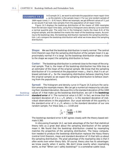
Figure 14.3 displays the bootstrap distribution of the means of 1000 resamples
from the Verizon repair time data, using first a histogram and a density curve and then
a normal quantile plot. The solid line in the histogram marks the mean 8.41 of the
original sample, and the dashed line marks the mean of the bootstrap means. According
to the bootstrap idea, the bootstrap distribution represents the sampling distribution.
Let’s compare the bootstrap distribution with what we know about the sampling
distribution.
Shape: We see that the bootstrap distribution is nearly normal. The central
limit theorem says that the sampling distribution of the sample mean x is approximately
normal if n is large. So the bootstrap distribution shape is close
to the shape we expect the sampling distribution to have.
Center: The bootstrap distribution is centered close to the mean of the original
sample. That is, the mean of the bootstrap distribution has little bias as
an estimator of the mean of the original sample. We know that the sampling
distribution of x is centered at the population mean µ, that is, that x is an unbiased
estimate of µ. So the resampling distribution behaves (starting from
the original sample) as we expect the sampling distribution to behave (starting
from the population).
bootstrap
standard error
Spread: The histogram and density curve in Figure 14.3 picture the variation
among the resample means. We can get a numerical measure by calculating
their standard deviation. Because this is the standard deviation of the 1000
values of x that make up the bootstrap distribution, we call it the bootstrap
standard error of x. The numerical value is 0.367. In fact, we know that the
standard deviation of x is σ/ √ n, where σ is the standard deviation of individual
observations in the population. Our usual estimate of this quantity is
the standard error of x, s/ √ n, where s is the standard deviation of our one
random sample. For these data, s = 14.69 and
s
√ n
= 14.69 √
1664
= 0.360
The bootstrap standard error 0.367 agrees closely with the theory-based estimate
0.360.
In discussing Example 14.2, we took advantage of the fact that statistical
theory tells us a great deal about the sampling distribution of the sample
mean x. We found that the bootstrap distribution created by resampling
matches the properties of the sampling distribution. The heavy computation
needed to produce the bootstrap distribution replaces the heavy theory
(central limit theorem, mean and standard deviation of x) that tells us about
the sampling distribution. The great advantage of the resampling idea is that it
often works even when theory fails. Of course, theory also has its advantages:
we know exactly when it works. We don’t know exactly when resampling
works, so that “When can I safely bootstrap?” is a somewhat subtle issue.