Chapter 14 - Bootstrap Methods and Permutation Tests - WH Freeman
Chapter 14 - Bootstrap Methods and Permutation Tests - WH Freeman
Chapter 14 - Bootstrap Methods and Permutation Tests - WH Freeman

You also want an ePaper? Increase the reach of your titles
YUMPU automatically turns print PDFs into web optimized ePapers that Google loves.
<strong>14</strong>-<strong>14</strong> CHAPTER <strong>14</strong> <strong>Bootstrap</strong> <strong>Methods</strong> <strong>and</strong> <strong>Permutation</strong> <strong>Tests</strong><br />
bias<br />
bootstrap<br />
estimate of bias<br />
• Center: A statistic is biased as an estimate of the parameter if its sampling<br />
distribution is not centered at the true value of the parameter. We<br />
can check bias by seeing whether the bootstrap distribution of the statistic<br />
is centered at the value of the statistic for the original sample.<br />
More precisely, the bias of a statistic is the difference between the mean<br />
of its sampling distribution <strong>and</strong> the true value of the parameter. The bootstrap<br />
estimate of bias is the difference between the mean of the bootstrap<br />
distribution <strong>and</strong> the value of the statistic in the original sample.<br />
• Spread: The bootstrap st<strong>and</strong>ard error of a statistic is the st<strong>and</strong>ard deviation<br />
of its bootstrap distribution. The bootstrap st<strong>and</strong>ard error estimates<br />
the st<strong>and</strong>ard deviation of the sampling distribution of the statistic.<br />
<strong>Bootstrap</strong> t confidence intervals<br />
If the bootstrap distribution of a statistic shows a normal shape <strong>and</strong> small<br />
bias, we can get a confidence interval for the parameter by using the bootstrap<br />
st<strong>and</strong>ard error <strong>and</strong> the familiar t distribution. An example will show how<br />
this works.<br />
We are interested in the selling prices of residential real estate in<br />
EXAMPLE <strong>14</strong>.4<br />
Seattle, Washington. Table <strong>14</strong>.1 displays the selling prices of a r<strong>and</strong>om<br />
sample of 50 pieces of real estate sold in Seattle during 2002, as recorded by the<br />
county assessor. 6 Unfortunately, the data do not distinguish residential property from<br />
commercial property. Most sales are residential, but a few large commercial sales in<br />
a sample can greatly increase the sample mean selling price.<br />
Figure <strong>14</strong>.6 shows the distribution of the sample prices. The distribution is far<br />
from normal, with a few high outliers that may be commercial sales. The sample is<br />
small, <strong>and</strong> the distribution is highly skewed <strong>and</strong> “contaminated” by an unknown number<br />
of commercial sales. How can we estimate the center of the distribution despite<br />
these difficulties?<br />
The first step is to ab<strong>and</strong>on the mean as a measure of center in favor of a<br />
statistic that is more resistant to outliers. We might choose the median, but<br />
in this case we will use a new statistic, the 25% trimmed mean.<br />
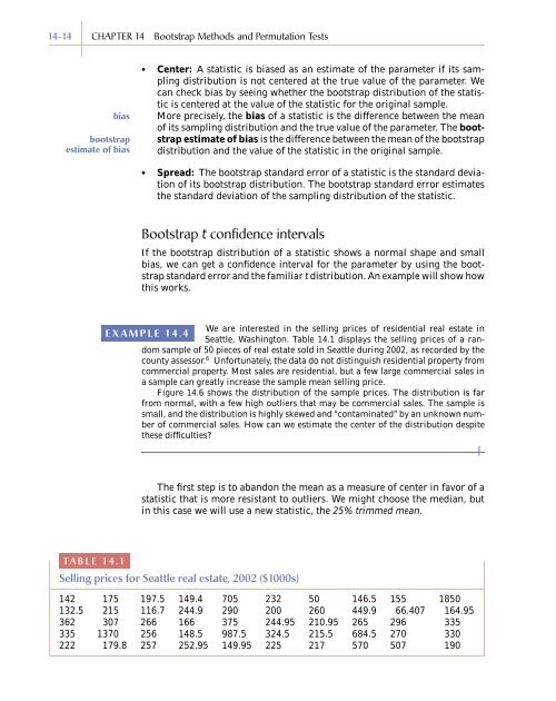
TABLE <strong>14</strong>.1<br />
Sellingprices for Seattle real estate, 2002 ($1000s)<br />
<strong>14</strong>2 175 197.5 <strong>14</strong>9.4 705 232 50 <strong>14</strong>6.5 155 1850<br />
132.5 215 116.7 244.9 290 200 260 449.9 66.407 164.95<br />
362 307 266 166 375 244.95 210.95 265 296 335<br />
335 1370 256 <strong>14</strong>8.5 987.5 324.5 215.5 684.5 270 330<br />
222 179.8 257 252.95 <strong>14</strong>9.95 225 217 570 507 190