Chapter 14 - Bootstrap Methods and Permutation Tests - WH Freeman

14-8 CHAPTER 14 Bootstrap Methods and Permutation Tests
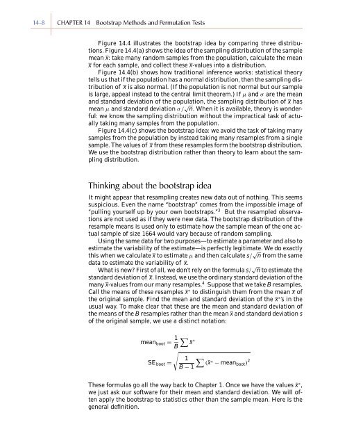
Figure 14.4 illustrates the bootstrap idea by comparing three distributions.
Figure 14.4(a) shows the idea of the sampling distribution of the sample
mean x: take many random samples from the population, calculate the mean
x for each sample, and collect these x-values into a distribution.
Figure 14.4(b) shows how traditional inference works: statistical theory
tells us that if the population has a normal distribution, then the sampling distribution
of x is also normal. (If the population is not normal but our sample
is large, appeal instead to the central limit theorem.) If µ and σ are the mean
and standard deviation of the population, the sampling distribution of x has
mean µ and standard deviation σ/ √ n. When it is available, theory is wonderful:
we know the sampling distribution without the impractical task of actually
taking many samples from the population.
Figure 14.4(c) shows the bootstrap idea: we avoid the task of taking many
samples from the population by instead taking many resamples from a single
sample. The values of x from these resamples form the bootstrap distribution.
We use the bootstrap distribution rather than theory to learn about the sampling
distribution.
Thinking about the bootstrap idea
It might appear that resampling creates new data out of nothing. This seems
suspicious. Even the name “bootstrap” comes from the impossible image of
“pulling yourself up by your own bootstraps.” 3 But the resampled observations
are not used as if they were new data. The bootstrap distribution of the
resample means is used only to estimate how the sample mean of the one actual
sample of size 1664 would vary because of random sampling.
Using the same data for two purposes—to estimate a parameter and also to
estimate the variability of the estimate—is perfectly legitimate. We do exactly
this when we calculate x to estimate µ and then calculate s/ √ n from the same
data to estimate the variability of x.
What is new? First of all, we don’t rely on the formula s/ √ n to estimate the
standard deviation of x. Instead, we use the ordinary standard deviation of the
many x-values from our many resamples. 4 Suppose that we take B resamples.
Call the means of these resamples ¯x ∗ to distinguish them from the mean x of
the original sample. Find the mean and standard deviation of the ¯x ∗ ’s in the
usual way. To make clear that these are the mean and standard deviation of
the means of the B resamples rather than the mean x and standard deviation s
of the original sample, we use a distinct notation:
mean boot = 1 ∑
¯x
∗
B
√
1 ∑
SE boot =
(¯x∗ − mean boot ) 2
B − 1
These formulas go all the way back to Chapter 1. Once we have the values ¯x ∗ ,
we just ask our software for their mean and standard deviation. We will often
apply the bootstrap to statistics other than the sample mean. Here is the
general definition.