- Page 1 and 2:
Public Economics Lectures Part 1: I
- Page 3 and 4:
Motivation 1: Practical Relevance I
- Page 5 and 6:
Motivation 2: Academic Interest Pub
- Page 7 and 8:
Methodological Themes 1 Micro-based
- Page 9 and 10:
Federal Government Revenue and Expe
- Page 11 and 12:
Federal Revenues (% of total revenu
- Page 13 and 14:
Federal Spending (% of total spendi
- Page 15 and 16:
Government Intervention in the Econ
- Page 17 and 18:
First Role for Government: Improve
- Page 19 and 20:
First Welfare Theorem Private marke
- Page 21 and 22:
Failure 2: Asymmetric Information a
- Page 23 and 24:
Individual Failures Recent addition
- Page 25 and 26:
Why Limit Government Intervention?
- Page 27 and 28:
Three Types of Questions in Public
- Page 29 and 30:
Public Economics Lectures Part 2: I
- Page 31 and 32:
References on Tax Incidence Kotliko
- Page 33 and 34:
Economic vs. Statutory Incidence Eq
- Page 35 and 36:
Overview of Literature Ideally, we
- Page 37 and 38:
Partial Equilibrium Model: Setup Tw
- Page 39 and 40:
Partial Equilibrium Model: Supply P
- Page 41 and 42:
Tax Levied on Producers Price S+t $
- Page 43 and 44:
Perfectly Inelastic Demand Price D
- Page 45 and 46:
Formula for Tax Incidence Implicitl
- Page 47 and 48:
Tax Incidence with Salience Effects
- Page 49 and 50:
Chetty et al.: Empirical Framework
- Page 51 and 52:
Chetty et al.: Strategy 1 Experimen
- Page 53 and 54:
TABLE 1 Evaluation of Tags: Classro
- Page 55 and 56:
Period Effect of Posting TaxInclu
- Page 57 and 58:
Period Effect of Posting TaxInclu
- Page 59 and 60:
Chetty et al.: Strategy 2 Compare e
- Page 61 and 62:
Per Capita Beer Consumption and Sta
- Page 63 and 64:
Tax Incidence with Salience Effects
- Page 65 and 66:
Tax Incidence with Salience Effects
- Page 67 and 68:
Evaluating Empirical Studies Consid
- Page 69 and 70:
Cigarette Taxation: Background Ciga
- Page 71 and 72:
Evans, Ringel, and Stech (1999) Exp
- Page 73 and 74:
Public Economics Lectures () Part 2
- Page 75 and 76:
Triple Difference Some studies use
- Page 77 and 78:
Fixed Effects Include time and stat
- Page 79 and 80:
Evans, Ringel, and Stech (1999) Imp
- Page 81 and 82:
Evans, Ringel, and Stech: Incidence
- Page 83 and 84:
Evans, Ringel, and Stech: Demand El
- Page 85 and 86:
Evans, Ringel, and Stech: Long Run
- Page 87 and 88:
Public Economics Lectures () Part 2
- Page 89 and 90:
Hastings and Washington 2008 Questi
- Page 91 and 92:
Public Economics Lectures () Part 2
- Page 93 and 94:
Public Economics Lectures () Part 2
- Page 95 and 96:
Rothstein 2008 How does EITC affect
- Page 97 and 98:
Public Economics Lectures () Part 2
- Page 99 and 100:
Rothstein: Empirical Strategy Two m
- Page 101 and 102:
DFL Reweighting Widely used method
- Page 103 and 104:
Public Economics Lectures () Part 2
- Page 105 and 106:
Public Economics Lectures () Part 2
- Page 107 and 108:
Rothstein: Results Basic DFL compar
- Page 109 and 110:
Rothstein: Results Ultimately uses
- Page 111 and 112:
Extensions of Basic Partial Equilib
- Page 113 and 114:
Extensions of Basic Partial Equilib
- Page 115 and 116:
Harberger 1962 Two Sector Model 1 F
- Page 117 and 118:
Harberger Model: Effect of Tax Incr
- Page 119 and 120:
Harberger Model: Main Effects 2. Ou
- Page 121 and 122:
Harberger Model: Main Effects 3. Su
- Page 123 and 124:
Computable General Equilibrium Mode
- Page 125 and 126:
Criticism of CGE Models Findings ve
- Page 127 and 128:
Open Economy Application: Framework
- Page 129 and 130:
Open Economy Application: Empirics
- Page 131 and 132:
Feldstein and Horioka 1980 Second s
- Page 133 and 134:
Open Economy Applications: Empirics
- Page 135 and 136:
Capitalization and the Asset Price
- Page 137 and 138:
Empirical Applications 1 [Cutler 19
- Page 139 and 140:
Cutler 1988 First, compute excess r
- Page 141 and 142:
Cutler: Results Cutler finds ˆb =
- Page 143 and 144:
Public Economics Lectures () Part 2
- Page 145 and 146:
Public Economics Lectures () Part 2
- Page 147 and 148:
Linden and Rockoff: Results Find ho
- Page 149 and 150:
Excess Returns Around Drug Approval
- Page 151 and 152:
Distribution of Excess Returns arou
- Page 153 and 154:
Mandated Benefits We have focused u
- Page 155 and 156:
Mandated Benefits: Simple Model Lab
- Page 157 and 158:
Mandated Benefit Wage Rate S w 1 B
- Page 159 and 160:
Mandated Benefits: Incidence Formul
- Page 161 and 162:
Gruber 1994 Studies state mandates
- Page 163 and 164:
Public Economics Lectures () Part 2
- Page 165 and 166:
Acemoglu and Angrist 2001 Look at e
- Page 167 and 168:
Acemoglu and Angrist 2001 Acemoglu
- Page 169 and 170:
Public Economics Lectures () Part 2
- Page 171 and 172:
Public Economics Lectures Part 3: E
- Page 173 and 174:
Definition Incidence analysis: effe
- Page 175 and 176:
Effi ciency Cost: Introduction Gove
- Page 177 and 178:
Partial Equilibrium Model: Setup Tw
- Page 179 and 180:
Price Excess Burden of Taxation S $
- Page 181 and 182:
Effi ciency Cost: Marshallian Surpl
- Page 183 and 184:
Effi ciency Cost: Marshallian Surpl
- Page 185 and 186:
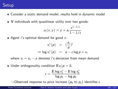
Effi ciency Cost: Marshallian Surpl
- Page 187 and 188:
EB Increases with Square of Tax Rat
- Page 189 and 190:
P P 3 P 2 P 1 S+t 1 +t 2 S+t 1 E B
- Page 191 and 192:
Tax Policy Implications With many g
- Page 193 and 194:
General Model: Demand and Indirect
- Page 195 and 196:
Path Dependence Problem Initial pri
- Page 197 and 198:
Consumer Surplus: Conceptual Proble
- Page 199 and 200:
Compensating and Equivalent Variati
- Page 201 and 202:
Equivalent Variation Measures utili
- Page 203 and 204:
Effi ciency Cost Formulas with Inco
- Page 205 and 206:
Compensating vs. Equivalent Variati
- Page 207 and 208:
Marshallian Surplus p h(V(p 1 ,Z))
- Page 209 and 210:
Excess Burden Deadweight burden: ch
- Page 211 and 212:
p h(V(p 1 ,Z)) ~ h(V(p 0 ,Z)) p 1 M
- Page 213 and 214:
Implementable Excess Burden Formula
- Page 215 and 216:
Harberger Formula Without pre-exist
- Page 217 and 218:
Goulder and Williams 2003 Show that
- Page 219 and 220:
Goulder and Williams Formula Obtain
- Page 221 and 222:
Goulder and Williams Results Calibr
- Page 223 and 224:
Harberger vs. Hausman Approach Unde
- Page 225 and 226:
Primitives Sufficient Stats. Welfar
- Page 227 and 228:
Heterogeneity Benefit of suff stat
- Page 229 and 230:
Discrete Choice Model Recast as pla
- Page 231 and 232:
Effi ciency Cost: Applications 1 [I
- Page 233 and 234:
Feldstein Model: Setup Government l
- Page 235 and 236:
Taxable Income Formula Simplicity o
- Page 237 and 238:
Excess Burden with Transfer Costs L
- Page 239 and 240:
Gorodnichenko, Martinez-Vazquez, an
- Page 241 and 242:
Public Economics Lectures () Part 3
- Page 243 and 244:
Poterba 1992 Estimates effi ciency
- Page 245 and 246:
Public Economics Lectures () Part 3
- Page 247 and 248:
Porterba: Results Tax reforms in 19
- Page 249 and 250:
Public Economics Lectures () Part 3
- Page 251 and 252:
Price and Tax Elasticities By Year
- Page 253 and 254:
Welfare Analysis in Behavioral Mode
- Page 255 and 256:
Behavioral Welfare Economics: Two A
- Page 257 and 258:
Behavioral Welfare Economics: Two A
- Page 259 and 260:
Bernheim and Rangel 2009: Choice Se
- Page 261 and 262:
Bernheim and Rangel 2009: Compensat
- Page 263 and 264:
Bernheim and Rangel 2009: Refinemen
- Page 265 and 266:
Welfare Analysis with Salience Effe
- Page 267 and 268:
Welfare Analysis with Salience Effe
- Page 269 and 270:
Preference Recovery Assumptions A1
- Page 271 and 272:
Excess Burden with No Income Effect
- Page 273 and 274:
Effi ciency Cost with Income Effect
- Page 275 and 276:
Directions for Further Work on Beha
- Page 277 and 278:
Outline 1 Commodity Taxation I: Ram
- Page 279 and 280:
Second Welfare Theorem Starting poi
- Page 281 and 282:
Four Central Results in Optimal Tax
- Page 283 and 284:
Ramsey Model: Key Assumptions 1 Lum
- Page 285 and 286:
Ramsey Model: Consumer Behavior Lag
- Page 287 and 288:
Ramsey Model: Government’s Proble
- Page 289 and 290:
Ramsey Formula: Perturbation Argume
- Page 291 and 292:
Ramsey Formula: Compensated Elastic
- Page 293 and 294:
Special Case 1: Inverse Elasticity
- Page 295 and 296:
Special Case 2: Uniform Taxation Th
- Page 297 and 298:
Diamond 1975: Many-Person Model H i
- Page 299 and 300:
Diamond: Many-Person Optimal Tax Fo
- Page 301 and 302:
Diamond: Optimal Transfer In this m
- Page 303 and 304:
Lipsey and Lancaster (1956): Theory
- Page 305 and 306:
Diamond and Mirrlees Model Two good
- Page 307 and 308:
Consumer’s Offer Curve Public Eco
- Page 309 and 310:
Production Set with Revenue Require
- Page 311 and 312:
Second Best: Optimal Distortionary
- Page 313 and 314:
Diamond and Mirrlees: General Model
- Page 315 and 316:
Proof of Production Effi ciency Res
- Page 317 and 318:
Policy Consequences: Public Sector
- Page 319 and 320:
Policy Consequences: No Taxation of
- Page 321 and 322:
Policy Consequences: No Taxation of
- Page 323 and 324:
Diamond and Mirrlees: Optimal Tax R
- Page 325 and 326:
Diamond and Mirrlees Result: Limita
- Page 327 and 328:
Key Concepts for Taxes/Transfers Le
- Page 329 and 330:
Optimal Income Tax with No Behavior
- Page 331 and 332:
Mirrlees 1971: Incorporating Behavi
- Page 333 and 334:
Mirrlees: Subsequent Work Mirrlees
- Page 335 and 336:
Revenue-Maximizing Tax Rate: Laffer
- Page 337 and 338:
Public Economics Lectures () Part 4
- Page 339 and 340:
Optimal Top Income Tax Rate { } dM
- Page 341 and 342:
Optimal Top Income Tax Rate In US t
- Page 343 and 344:
Connection to Revenue Maximizing Ta
- Page 345 and 346:
Public Economics Lectures () Part 4
- Page 347 and 348:
General Non-Linear Income Tax Optim
- Page 349 and 350:
Numerical Simulations of Optimal Ta
- Page 351 and 352:
Numerical Simulations Use formula e
- Page 353 and 354:
Commodity vs. Income Taxation Now c
- Page 355 and 356:
Atkinson and Stiglitz: Commodity Ta
- Page 357 and 358:
Atkinson-Stiglitz: Proof Revenue un
- Page 359 and 360:
Atkinson-Stiglitz: Intuition With s
- Page 361 and 362:
Atkinson-Stiglitz: Implications for
- Page 363 and 364:
Chamley-Judd: Capital Taxation Judd
- Page 365 and 366:
Taxation and Savings: Evidence Key
- Page 367 and 368:
Public Economics Lectures () Part 4
- Page 369 and 370:
Optimal Transfer Programs Several t
- Page 371 and 372:
Optimal Transfers: Mirrless Model M
- Page 373 and 374:
Saez 2002: Participation Model Mode
- Page 375 and 376:
Public Economics Lectures () Part 4
- Page 377 and 378:
Public Economics Lectures () Part 4
- Page 379 and 380:
Saez 2002: Optimal Tax Formula Smal
- Page 381 and 382:
Public Economics Lectures () Part 4
- Page 383 and 384:
Public Economics Lectures () Part 4
- Page 385 and 386:
Public Economics Lectures () Part 4
- Page 387 and 388:
Mankiw and Weinzierl 2009 Tagging w
- Page 389 and 390:
Nichols and Zeckhauser 1982: In-Kin
- Page 391 and 392:
Soup Kitchen without Wait: Cash Tra
- Page 393 and 394:
Income Taxation as Insurance (Varia
- Page 395 and 396:
Varian Model: Private Insurance Var
- Page 397 and 398:
Public Economics Lectures Part 5: I
- Page 399 and 400:
References Surveys in labor economi
- Page 401 and 402:
Baseline Labor-Leisure Choice Model
- Page 403 and 404:
Labor Supply Behavior First order c
- Page 405 and 406:
Econometric Problem 1: Unobserved H
- Page 407 and 408:
Measurement Error and Division Bias
- Page 409 and 410:
Extensive vs. Intensive Margin Rela
- Page 411 and 412:
Progressive Taxes and Labor Supply
- Page 413 and 414:
Example 1: Progressive Income Tax P
- Page 415 and 416:
Example 3: Social Security Payroll
- Page 417 and 418:
Progressive Taxes and Labor Supply
- Page 419 and 420:
Non-Linear Budget Set Estimation: V
- Page 421 and 422:
Likelihood Function: Located at the
- Page 423 and 424:
Hausman (1981) Application Hausman
- Page 425 and 426:
Saez 2009: Bunching at Kinks Saez o
- Page 427 and 428:
Public Economics Lectures ()Part 5:
- Page 429 and 430:
Earnings Density and the EITC: Wage
- Page 431 and 432:
Taxable Income Density, 1960-1969:
- Page 433 and 434:
Friedberg 2000: Social Security Ear
- Page 435 and 436:
Friedberg: Estimates Estimates elas
- Page 437 and 438:
Public Economics Lectures ()Part 5:
- Page 439 and 440:
Why not more bunching at kinks? 1 T
- Page 441 and 442:
Public Economics Lectures ()Part 5:
- Page 443 and 444:
Chetty et al. 2009: Model Firms pos
- Page 445 and 446:
Cost of Bunching at Bracket Cutoff
- Page 447 and 448:
Marginal Tax Rates in Denmark in 19
- Page 449 and 450:
All Wage Earners: Top Tax Bracket C
- Page 451 and 452:
Married Women Frequency 0 10000 200
- Page 453 and 454:
Married Female Professionals with A
- Page 455 and 456:
Married Women, 1994 Frequency 0 100
- Page 457 and 458:
Married Women, 1996 Frequency 0 100
- Page 459 and 460:
Married Women, 1998 Frequency 0 100
- Page 461 and 462:
Married Women, 2000 Frequency 0 100
- Page 463 and 464:
Married Women at the Middle Tax: 10
- Page 465 and 466:
Married Women at the Middle Tax: 8%
- Page 467 and 468:
Distribution of Individuals’Deduc
- Page 469 and 470:
Teachers Wage Income: 1998 Frequenc
- Page 471 and 472:
Wage Earnings: Teachers with Deduct
- Page 473 and 474:
Distribution of Modes in Occupation
- Page 475 and 476:
SelfEmployed: Distribution around
- Page 477 and 478:
Estimates of Hours and Participatio
- Page 479 and 480:
Public Economics Lectures ()Part 5:
- Page 481 and 482:
Public Economics Lectures ()Part 5:
- Page 483 and 484:
Problems with Experimental Design E
- Page 485 and 486:
Instrumental Variable Methods Anoth
- Page 487 and 488:
Mroz 1987: Setup and Results Uses b
- Page 489 and 490:
Public Economics Lectures ()Part 5:
- Page 491 and 492:
Public Economics Lectures ()Part 5:
- Page 493 and 494:
Eissa 1995: Caveats Does the common
- Page 495 and 496:
Bianchi, Gudmundsson, and Zoega 200
- Page 497 and 498:
Public Economics Lectures ()Part 5:
- Page 499 and 500:
Bianchi, Gudmundsson, and Zoega 200
- Page 501 and 502:
Overall Costs of Anti Poverty Progr
- Page 503 and 504:
Monthly Welfare Case Loads: 1963-20
- Page 505 and 506:
Behavioral Responses to the EITC 1
- Page 507 and 508:
Eissa and Liebman 1996 Study labor
- Page 509 and 510:
Eissa and Liebman: Results Find a s
- Page 511 and 512:
Public Economics Lectures ()Part 5:
- Page 513 and 514:
Meyer and Rosenbaum 2001 Analyze th
- Page 515 and 516:
Eissa and Hoynes 2004 EITC based on
- Page 517 and 518:
Meyer and Sullivan 2004 Examine the
- Page 519 and 520:
Relative Consumption: single women
- Page 521 and 522:
Meyer and Sullivan: Results Materia
- Page 523 and 524:
Changing Elasticities: Blau and Kah
- Page 525 and 526:
Intertemporal Models and the MaCurd
- Page 527 and 528:
Life Cycle Model: Time Separability
- Page 529 and 530: Dynamic Life Cycle Model: Frisch El
- Page 531 and 532: Public Economics Lectures ()Part 5:
- Page 533 and 534: Frisch vs. Compensated vs. Uncompen
- Page 535 and 536: Card Critique of ITLS models Critiq
- Page 537 and 538: Blundell, Duncan, and Meghir 1998 C
- Page 539 and 540: Blundell, Duncan, and Meghir: Resul
- Page 541 and 542: Public Economics Lectures ()Part 5:
- Page 543 and 544: Farber 2005: Division Bias Argues t
- Page 545 and 546: Manoli and Weber 2009 Use variation
- Page 547 and 548: Distribution of Tenure at Retiremen
- Page 549 and 550: US Income Taxation: Trends The bigg
- Page 551 and 552: Bottom 99% Tax Units 40% $40,000 35
- Page 553 and 554: Feldstein 1995 First study of taxab
- Page 555 and 556: Feldstein: Results Feldstein obtain
- Page 557 and 558: Feldstein: Econometric Criticisms S
- Page 559 and 560: 18% 16% Wages SCorp. Partner. Sol
- Page 561 and 562: Public Economics Lectures ()Part 5:
- Page 563 and 564: Gruber and Saez 2002 First study to
- Page 565 and 566: Gruber and Saez: Results Find an el
- Page 567 and 568: Imbens et al. 2001: Income Effects
- Page 569 and 570: Taxable Income Literature: Summary
- Page 571 and 572: Prescott 2004 Uses data on hours wo
- Page 573 and 574: Davis and Henrekson 2005 Run regres
- Page 575 and 576: Public Economics Lectures ()Part 5:
- Page 577 and 578: Optimization Frictions Many frictio
- Page 579: Public Economics Lectures ()Part 5:
- Page 583 and 584: Optimization Frictions Define agent
- Page 585 and 586: Construction of Choice Set 151 150
- Page 587 and 588: Identification with Optimization Fr
- Page 589 and 590: Identification with Optimization Fr
- Page 591 and 592: Calculation of Bounds on Structural
- Page 593 and 594: ) Lower Bound on Structural Elastic
- Page 595 and 596: Application to Taxation and Labor S
- Page 597 and 598: 4.0 Bounds on IntensiveMargin Lab
- Page 599 and 600: 4.0 3.5 Bounds on IntensiveMargin
- Page 601 and 602: Chetty and Saez 2009: Experimental
- Page 603 and 604: Year 2 Earnings Distributions: 1 De
- Page 605 and 606: Year 2 Wage Earnings Distributions:
- Page 607 and 608: Labor Supply Elasticities: Implicat
- Page 609 and 610: Chetty: Formula for Risk Aversion L
- Page 611 and 612: u c ,u l w 0 u c (w 0 l,l) Case A:
- Page 613 and 614: Chetty 2006: Results Labor supply e
- Page 615 and 616: Outline 1 Motivations for Social In
- Page 617 and 618: Growth of Social Insurance in the U
- Page 619 and 620: Unemployment Benefit Systems in Dev
- Page 621 and 622: Useful Background Reading 1 Institu
- Page 623 and 624: Adverse Selection as a Motivation f
- Page 625 and 626: Rothschild-Stiglitz: Key Assumption
- Page 627 and 628: Rothschild-Stiglitz: Equilibrium De
- Page 629 and 630: Public Economics Lectures () Part 6
- Page 631 and 632:
Rothschild-Stiglitz: Second Best So
- Page 633 and 634:
Rothschild-Stiglitz: Second Best So
- Page 635 and 636:
Rothschild-Stiglitz: Second Best So
- Page 637 and 638:
Rothschild-Stiglitz: Second Best So
- Page 639 and 640:
Adverse Selection: Empirical Eviden
- Page 641 and 642:
Public Economics Lectures () Part 6
- Page 643 and 644:
Aggregate Shocks as a Motivation fo
- Page 645 and 646:
Unemployment Insurance Start with U
- Page 647 and 648:
Replacement Rate Common measure of
- Page 649 and 650:
Baily-Chetty model Canonical analys
- Page 651 and 652:
Baily-Chetty model: Setup Static mo
- Page 653 and 654:
Baily-Chetty model: First Best Prob
- Page 655 and 656:
Baily-Chetty model: Second Best Pro
- Page 657 and 658:
Two Approaches to Optimal Social In
- Page 659 and 660:
Envelope Condition Why can ∂e ∂
- Page 661 and 662:
Suffi cient Statistic Approach to K
- Page 663 and 664:
Baily-Chetty model: Second Best Sol
- Page 665 and 666:
Baily-Chetty Consumption-Based Form
- Page 667 and 668:
Empirical Estimates: Duration Elast
- Page 669 and 670:
Hazard Models Define hazard rate h
- Page 671 and 672:
Meyer 1990 Meyer includes log UI be
- Page 673 and 674:
Consumption Smoothing Benefits of U
- Page 675 and 676:
Consumption Smoothing Benefits of U
- Page 677 and 678:
Calibrating the Model b ∗ Results
- Page 679 and 680:
Homeowners’Consumption around Une
- Page 681 and 682:
Commitments and Risk Aversion How d
- Page 683 and 684:
Commitments Model: Implications for
- Page 685 and 686:
Chetty 2008: Moral Hazard vs. Liqui
- Page 687 and 688:
Chetty 2008: Job Search Technology
- Page 689 and 690:
Chetty 2008: Value Functions Value
- Page 691 and 692:
Chetty 2008: Moral Hazard vs. Liqui
- Page 693 and 694:
Chetty 2008: Formula for Optimal UI
- Page 695 and 696:
Moral Hazard vs. Liquidity: Evidenc
- Page 697 and 698:
Figure 3a Effect of UI Benefits on
- Page 699 and 700:
Figure 3c Effect of UI Benefits on
- Page 701 and 702:
log UI ben 0.527 (0.267) TABLE 2
- Page 703 and 704:
Figure 5 Effect of Severance Pay on
- Page 705 and 706:
Figure 6b Effect of Severance Pay o
- Page 707 and 708:
Chetty 2008: Implications for Optim
- Page 709 and 710:
Figure 3 Frequency of Layoffs by Jo
- Page 711 and 712:
Figure 4 Selection on Observables M
- Page 713 and 714:
TABLE 3a Effects of Severance Pay a
- Page 715 and 716:
Shimer and Werning 2007: Reservatio
- Page 717 and 718:
Figure 5a Effect of Severance Pay o
- Page 719 and 720:
Figure 10b Effect of Severance Pay
- Page 721 and 722:
Effect of Extended Benefits on Subs
- Page 723 and 724:
Spike at Benefit Exhaustion Most st
- Page 725 and 726:
Job Finding vs. Unemployment Exit H
- Page 727 and 728:
Effect of Benefit Expiration on Haz
- Page 729 and 730:
Experience Rating in Washington, 20
- Page 731 and 732:
Feldstein 1978: Empirical Results F
- Page 733 and 734:
UI Savings Accounts Alternative to
- Page 735 and 736:
Feldstein and Altman 2007 Calculati
- Page 737 and 738:
Black, Smith, Berger, and Noel 2003
- Page 739 and 740:
Public Economics Lectures () Part 6
- Page 741 and 742:
Black, Smith, Berger, and Noel 2003
- Page 743 and 744:
Dynamics: Path of UI Benefits Class
- Page 745 and 746:
Workers Compensation Insurance agai
- Page 747 and 748:
Theory of Workers’Compensation Fo
- Page 749 and 750:
Public Economics Lectures () Part 6
- Page 751 and 752:
Effects of Benefits on Injuries Pot
- Page 753 and 754:
Public Economics Lectures () Part 6
- Page 755 and 756:
Effect on Equilibrium Wage Workers
- Page 757 and 758:
Disability Insurance See Bound et.
- Page 759 and 760:
Two Views on the Rise in DI Trend h
- Page 761 and 762:
Theory of Disability Insurance Key
- Page 763 and 764:
Empirical Evidence: Bound-Parsons D
- Page 765 and 766:
Empirical Evidence: Bound-Parsons D
- Page 767 and 768:
Gruber 2000 Exploits differential l
- Page 769 and 770:
Public Economics Lectures () Part 6
- Page 771 and 772:
Autor and Duggan 2003 Focus on inte
- Page 773 and 774:
Public Economics Lectures () Part 6
- Page 775 and 776:
Employment Shocks and DI Applicatio
- Page 777 and 778:
Employment Shocks and DI Applicatio
- Page 779 and 780:
Health Insurance Arrow (1963): semi
- Page 781 and 782:
Health Care Spending in OECD Nation
- Page 783 and 784:
Americans’Source of Health Insura
- Page 785 and 786:
Growing Health Expenditures: Key Fa
- Page 787 and 788:
Market Failures and Government Inte
- Page 789 and 790:
Measuring Health Before discussing
- Page 791 and 792:
Public Economics Lectures () Part 6
- Page 793 and 794:
Optimal Govt. Intervention in Healt
- Page 795 and 796:
Feldstein 1973 x = non-medical cons
- Page 797 and 798:
Feldstein 1973: First Best Solution
- Page 799 and 800:
Price of each visit $200 A B S=MC $
- Page 801 and 802:
Public Economics Lectures () Part 6
- Page 803 and 804:
Public Economics Lectures () Part 6
- Page 805 and 806:
Finkelstein 2006 Impact of Medicare
- Page 807 and 808:
Ellis and McGuire 1986 Previous ana
- Page 809 and 810:
Ellis and McGuire: Compensation Sch
- Page 811 and 812:
Ellis and McGuire: Optimal Payment
- Page 813 and 814:
Ellis and McGuire: Optimal Payment
- Page 815 and 816:
Ellis and McGuire Model: Limitation
- Page 817 and 818:
Crowdout of Private Insurance So fa
- Page 819 and 820:
Currie and Gruber 1995: Benefits of
- Page 821 and 822:
Public Economics Lectures Part 7: P
- Page 823 and 824:
Public vs. Private Goods Private go
- Page 825 and 826:
Public Good Person 1’s Consumptio
- Page 827 and 828:
Public Goods Model: Setup Economy w
- Page 829 and 830:
First Best if G is Private To ident
- Page 831 and 832:
First Best if G is a Pure Public Go
- Page 833 and 834:
Samuelson (1954) Rule Condition for
- Page 835 and 836:
Model of Private Provision: Setup P
- Page 837 and 838:
Lindahl Equilibrium How to achieve
- Page 839 and 840:
Lindahl Equilibria: Key Properties
- Page 841 and 842:
Voting Model: Setup Suppose that pu
- Page 843 and 844:
Arrow (1951) and Single-Peaked Pref
- Page 845 and 846:
Median Voter Theorem With single-pe
- Page 847 and 848:
Median Voter Choice: Effi ciency In
- Page 849 and 850:
Public Economics Lectures () Part 7
- Page 851 and 852:
Optimal Second Best Provision of PG
- Page 853 and 854:
Bergstrom, Blume, and Varian (1986)
- Page 855 and 856:
Bergstrom-Blume-Varian Model: Crowd
- Page 857 and 858:
BBV Model: Additional Results 1 Tot
- Page 859 and 860:
Empirical Evidence on Crowd-Out Two
- Page 861 and 862:
Public Economics Lectures () Part 7
- Page 863 and 864:
Hungerman 2005 Studies crowdout of
- Page 865 and 866:
Hungerman 2005 Estimates imply that
- Page 867 and 868:
Andreoni and Payne 2003 OLS still y
- Page 869 and 870:
Andreoni and Payne 2003 $1000 incre
- Page 871 and 872:
Public Economics Lectures () Part 7
- Page 873 and 874:
Andreoni 1988 Isaac, McCue, and Plo
- Page 875 and 876:
Andreoni 1993 Uses lab experiment t
- Page 877 and 878:
Public Economics Lectures () Part 7
- Page 879 and 880:
Andreoni 1993 Public good levels ar
- Page 881 and 882:
Financing PGs with Distortionary Ta
- Page 883 and 884:
PGs with Distortionary Taxes: Setup
- Page 885 and 886:
PGs with Distortionary Taxes: 1st B
- Page 887 and 888:
PGs with Distortionary Taxes: 2nd B
- Page 889 and 890:
Kreiner and Verdelin 2009 Consider
- Page 891 and 892:
Subsidies for Charity: Setup Warm-g
- Page 893 and 894:
Optimal Subsidies for Charity Resul
- Page 895 and 896:
Optimal Subsidies for Charity (Saez
- Page 897 and 898:
Empirical Evidence Existing studies
- Page 899 and 900:
Externalities: Outline 1 Definition
- Page 901 and 902:
Externalities: Main Questions 1 The
- Page 903 and 904:
Model of Externalities: Equilibrium
- Page 905 and 906:
Model of Externalities: Deadweight
- Page 907 and 908:
Remedies for Externalities 1 Coasia
- Page 909 and 910:
Coasian Solution: Limitations 1 Cos
- Page 911 and 912:
Price Pigouvian Tax SMC=PMC+MD S=PM
- Page 913 and 914:
Permits: Cap-and-Trade Cap total am
- Page 915 and 916:
Weitzman 1974: Market for Pollution
- Page 917 and 918:
Weitzman Model: Policy without Unce
- Page 919 and 920:
MB steep, Quantity regulation Publi
- Page 921 and 922:
Quantity Regulation Price Regulatio
- Page 923 and 924:
MB Flat, Quantity Regulation Public
- Page 925 and 926:
Quantity regulation Price Regulatio
- Page 927 and 928:
Optimal Second-Best Taxation with E
- Page 929 and 930:
Sandmo 1975: Setup Individual maxim
- Page 931 and 932:
Sandmo 1975: Additivity Result Main
- Page 933 and 934:
Double Dividend Debate Claim: gas t
- Page 935 and 936:
Externalities: Empirical Measuremen
- Page 937 and 938:
Public Economics Lectures () Part 7
- Page 939 and 940:
Public Economics Lectures () Part 7
- Page 941 and 942:
Brookshire et al. 1982 Infer willin
- Page 943 and 944:
Public Economics Lectures () Part 7
- Page 945 and 946:
Chay and Greenstone 2005 Conclusion
- Page 947 and 948:
Public Economics Lectures () Part 7
- Page 949 and 950:
Public Economics Lectures () Part 7
- Page 951 and 952:
Public Economics Lectures () Part 7
- Page 953 and 954:
Diamond and Hausman 1994 Describe p
- Page 955 and 956:
Becker and Murphy 1988 Show that ad
- Page 957 and 958:
Bernheim and Rangel 2004 Model of