

Self-Consistent Field Theory and Its Applications by M. W. Matsen
Self-Consistent Field Theory and Its Applications by M. W. Matsen
Self-Consistent Field Theory and Its Applications by M. W. Matsen

Create successful ePaper yourself
Turn your PDF publications into a flip-book with our unique Google optimized e-Paper software.
38 1 <strong>Self</strong>-consistent field theory <strong>and</strong> its applications<br />
where the elements of the diagonal matrix, d k ≡ D kk , are the eigenvalues of A <strong>and</strong> the respective<br />
columns of U are the corresponding normalized eigenvectors. Since A is symmetric,<br />
all the eigenvalues will be real <strong>and</strong> U −1 = U T . We can then express T(s) =U exp(Ds)U T ,<br />
from which it follows that<br />
T ij (s) = ∑ k<br />
exp(sd k )U ik U jk (1.176)<br />
Similarly, the solution for the complementary function, q † (z,s) ≡ ∑ i q† i (s)f i(z),isgiven<strong>by</strong><br />
q † i (s) =∑ j<br />
T ij (1 − s)q † j (1) (1.177)<br />
where<br />
q † i (1) = 1 L<br />
∫ L<br />
0<br />
(√ ) aN<br />
dzq † 1/2<br />
(z,1)f i (z) =C i cos λi<br />
L<br />
(1.178)<br />
This result is obtained <strong>by</strong> first integrating with q † (z,1) = aN 1/2 δ(z − ɛ), <strong>and</strong> then taking the<br />
limit, ɛ → 0. Once the partial partition functions are evaluated, the partition function for the<br />
entire chain is obtained <strong>by</strong><br />
Q[w]<br />
V<br />
= ∑ i<br />
q i (s)q † i (s) =∑ i<br />
exp(d i )¯q i (0)¯q † i (1) (1.179)<br />
where we have made the convenient definitions, ¯q i (0) ≡ ∑ j q j(0)U ji <strong>and</strong> ¯q † i (1) ≡ ∑ j q† j (1)U ji.<br />
2<br />
w(z) a2 N/L 2<br />
1<br />
0<br />
-1<br />
-2<br />
2<br />
4<br />
L/aN 1/2 = 1<br />
-3<br />
0.0 0.2 0.4 0.6 0.8 1.0<br />
z/L<br />
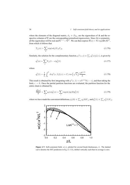
Figure 1.7: <strong>Self</strong>-consistent field, w(z), plotted for several brush thicknesses, L. The dashed<br />
curve denotes the SST prediction in Eq. (1.113), shifted vertically such that its average is zero.


