

Self-Consistent Field Theory and Its Applications by M. W. Matsen
Self-Consistent Field Theory and Its Applications by M. W. Matsen
Self-Consistent Field Theory and Its Applications by M. W. Matsen

Create successful ePaper yourself
Turn your PDF publications into a flip-book with our unique Google optimized e-Paper software.
1.8 Block Copolymer Melts 61<br />
1.2<br />
f = 0.5<br />
S(k)/N<br />
0.8<br />
0.4<br />
χN=10<br />
9<br />
8<br />
0.0<br />
0 2 4 6 8 10<br />
kaN 1/2<br />
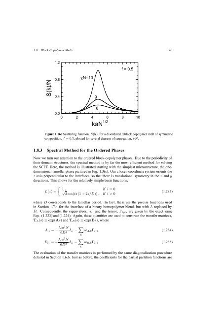
Figure 1.16: Scattering function, S(k), for a disordered diblock copolymer melt of symmetric<br />
composition, f =0.5, plotted for several degrees of segregation, χN.<br />
1.8.3 Spectral Method for the Ordered Phases<br />
Now we turn our attention to the ordered block-copolymer phases. Due to the periodicity of<br />
their domain structures, the spectral method is <strong>by</strong> far the most efficient method for solving<br />
the SCFT. Here, the method is illustrated starting with the simplest microstructure, the onedimensional<br />
lamellar phase pictured in Fig. 1.3(c). Our chosen coordinate system orients the<br />
z axis perpendicular to the interfaces, so that there is translational symmetry in the x <strong>and</strong> y<br />
directions. This allows for the relatively simple basis functions,<br />
f i (z) =<br />
{ 1 , if i =0<br />
√<br />
2cos(iπ(1 + 2z/D)) , if i>0<br />
(1.283)<br />
where D corresponds to the lamellar period. In fact, these are the precise functions used<br />
in Section 1.7.4 for the interface of a binary homopolymer blend, but with L replaced <strong>by</strong><br />
D. Consequently, the eigenvalues, λ i , <strong>and</strong> the tensor, Γ ijk , are given <strong>by</strong> the exact same<br />
Eqs. (1.223) <strong>and</strong> (1.224). Again, these quantities are used to construct the transfer matrices,<br />
T A (s) ≡ exp(As) <strong>and</strong> T B (s) ≡ exp(Bs), where<br />
A ij = − λ ia 2 N<br />
6D 2 δ ij − ∑ k<br />
B ij = − λ ia 2 N<br />
6D 2 δ ij − ∑ k<br />
w A,k Γ ijk (1.284)<br />
w B,k Γ ijk (1.285)<br />
The evaluation of the transfer matrices is performed <strong>by</strong> the same diagonalization procedure<br />
detailed in Section 1.6.6. Just as before, the coefficients for the partial partition functions are


