Self-Consistent Field Theory and Its Applications by M. W. Matsen

More documents

Recommendations

Info

1.1 Gaussian Chain 7 structure involving an extensive amount of internal interface. Naturally, the properties of the interface have a pronounced effect on the final material; in particular, a high interfacial tension results in large domains, which is generally undesirable. One way of halting the tendency of domains to coarsen is to chemically bond the unlike polymers together, forming block copolymer molecules. The blocks still segregate into separate domains, but the connectivity of the chain prevents the domains from becoming thicker than the typical size of a single molecule. In fact, the domains tend to form highly-ordered periodic geometrics, of which the lamellar phase of alternating thin layers pictured in Fig. 1.3(c) is the simplest. This ability to selfassemble into ordered nanoscale morphologies of different geometries is a powerful feature that researchers are now beginning to exploit for various high-tech applications. 1.1 Gaussian Chain To start off, we consider linear homopolymer chains in a homogeneous environment, and disregard, for the moment, all monomer-monomer interactions including the hard-core ones that prevent the chains from overlapping. In the limit of high molecular weights, all such polymers fall into the same universality class of non-avoiding random walks, and as a consequence they exhibit a degree of common behavior. For instance, their typical size scales with their molecular weight to the universal exponent, ν =1/2. To investigate this common behavior, there is no need to consider realistic polymer chains involving segments such as those denoted in Fig. 1.2. The fact that the behavior is universal means that it is exhibited by all models, including simple artificial ones. For maximum simplicity, we select the freely-jointed chain, where each monomer has a fixed length, b, and the joint between sequential monomers is completely flexible. Figure 1.4(a) shows a typical configuration of this model, projected onto the two-dimensional page. It was produced by joining together M = 4000 vectors, r i , each generated from the random distribution, p 1 (r i )= δ(r i − b) 4πb 2 (1.1) where r i ≡|r i |. The factor in the denominator ensures that the distribution is properly normalized such that ∫ ∫ ∞ dr p 1 (r) =4π dr r 2 p 1 (r) =1 (1.2) 0 The size of the particular configuration displayed in Fig. 1.4(a) can be characterized by the length of its end-to-end vector, R ≡ M∑ r i (1.3) i=1 denoted by the arrow at the top of the figure. The length of this vector averaged over all possible configurations, R 0 , can then be used as a measure for the typical size of the polymer.
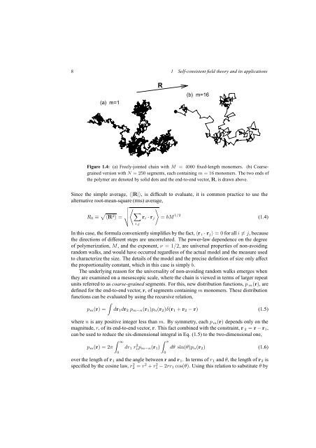
8 1 Self-consistent field theory and its applications (a) m=1 R (b) m=16 Figure 1.4: (a) Freely-jointed chain with M = 4000 fixed-length monomers. (b) Coarsegrained version with N = 250 segments, each containing m =16monomers. The two ends of the polymer are denoted by solid dots and the end-to-end vector, R, is drawn above. Since the simple average, 〈|R|〉, is difficult to evaluate, it is common practice to use the alternative root-mean-square (rms) average, R 0 ≡ √ 〈〉 ∑ 〈R 2 〉 = √ r i · r j = bM 1/2 (1.4) i,j In this case, the formula conveniently simplifies by the fact, 〈r i · r j 〉 =0for all i ≠ j, because the directions of different steps are uncorrelated. The power-law dependence on the degree of polymerization, M, and the exponent, ν =1/2, are universal properties of non-avoiding random walks, and would have occurred regardless of the actual model and the measure used to characterize the size. The details of the model and the precise definition of size only affect the proportionality constant, which in this case is simply b. The underlying reason for the universality of non-avoiding random walks emerges when they are examined on a mesoscopic scale, where the chain is viewed in terms of larger repeat units referred to as coarse-grained segments. For this, new distribution functions, p m (r), are defined for the end-to-end vector, r, of segments containing m monomers. These distribution functions can be evaluated by using the recursive relation, ∫ p m (r) = dr 1 dr 2 p m−n (r 1 )p n (r 2 )δ(r 1 + r 2 − r) (1.5) where n is any positive integer less than m. By symmetry, each p m (r) depends only on the magnitude, r, of its end-to-end vector, r. This fact combined with the constraint, r 2 = r − r 1 , can be used to reduce the six-dimensional integral in Eq. (1.5) to the two-dimensional one, p m (r) =2π ∫ ∞ 0 dr 1 r 2 1 p m−n(r 1 ) ∫ π 0 dθ sin(θ)p n (r 2 ) (1.6) over the length of r 1 and the angle between r and r 1 . In terms of r 1 and θ, the length of r 2 is specified by the cosine law, r 2 2 = r2 + r 2 1 − 2rr 1 cos(θ). Using this relation to substitute θ by
Page 1 and 2: Self-Consistent Field Theory and It
Page 3 and 4: 2 Contents Index 83
Page 5 and 6: 4 1 Self-consistent field theory an
Page 7: 6 1 Self-consistent field theory an
Page 11 and 12: 10 1 Self-consistent field theory a
Page 59 and 60:
58 1 Self-consistent field theory a
Page 61 and 62:
Page 63 and 64:
Page 65 and 66:
Page 67 and 68:
Page 69 and 70:
Page 71 and 72:
Page 73 and 74:
Page 75 and 76:
Page 77 and 78:
Page 80 and 81:
Bibliography Almdal, K., Rosedale,
Page 82 and 83:
BIBLIOGRAPHY 81 Matsen, M. W. and G
Page 84 and 85:
Index action 17 binodal point 46 bl
show all

Self-Consistent Field Theory and Its Applications by M. W. Matsen

You also want an ePaper? Increase the reach of your titles

Delete template?

Save as template?