Optimal Design of LCL Harmonic Filters for Three-Phase PFC ...

3116 IEEE TRANSACTIONS ON POWER ELECTRONICS, VOL. 28, NO. 7, JULY 2013
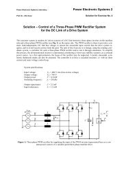
Fig. 2. Reluctance model of the inductor shown in Fig. 1(b). It consists of one
voltage source (representing the two separated windings), one air gap reluctance
R g (representing the two air gaps), and one core reluctance R c .
can only be solved iteratively by using a numerical method. In
the case at hand, the problem has been solved by applying the
Newton approach.
The reluctance model of the inductor shown in Fig. 1(b) is
illustrated in Fig. 2. It consists of one voltage source (representing
the two separated windings), one air gap reluctance R g
(representing the two air gaps), and one core reluctance R c .The
fact that the flux density in core parts very close to the air gap is
(slightly) reduced as the flux lines already left the core has been
neglected.
B. Core Losses
The applied core loss approach is described in [10] in detail
and can be seen as a hybrid of the improved–improved Generalized
Steinmetz Equation i 2 GSE [12] and a loss map approach:
a loss map is experimentally determined and the interpolation
and extrapolation for operating points in between the measured
values is then made with the i 2 GSE.
The flux density waveform for which the losses have to be
calculated is, e.g., simulated in a circuit simulator, where the
magnetic part is modeled as a reluctance model. This simulated
waveform is then divided into its fundamental flux waveform
and into piecewise linear flux waveform segments. The loss
energy is then derived for the fundamental and all piecewise
linear segments, summed up and divided by the fundamental
period length in order to determine the average core loss. The dc
flux level of each piecewise linear flux segment is considered, as
this influences the core losses [13]. Furthermore, the relaxation
term of the i 2 GSE is evaluated for each transition from one
piecewise linear flux segment to another.
Another aspect to be considered in the core loss calculation
is the effect of the core shape/size. By introducing a reluctance
model of the core, the flux density can be calculated. Subsequently,
for each core section with (approximately) homogenous
flux density, the losses can be determined. In the case at
hand, the core has been divided into four straight core sections
and four corner sections. The core losses of the sections are then
summed up to obtain the total core losses.
C. Winding Losses
The second source of losses in inductive components is the
ohmic losses in the windings. The resistance of a conductor
increases with increasing frequency due to eddy currents. Selfinduced
eddy currents inside a conductor lead to the skin effect.
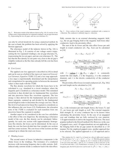
Fig. 3. Cross section of the round conductor considered with a current in
z-direction. The conductor is infinitely large in z-direction.
Eddy currents due to an external alternating magnetic field,
e.g., the air gap fringing field or the magnetic field from other
conductors, lead to the proximity effect.
The sum of the dc losses and the skin effect losses per unit
length in round conductors [cf., Fig. 3(a)] can be calculated
as [14]
and 1 F R (f) = ξ
4 √ 2
with δ =
1 √ πμ0 σf ,ξ =
P S = R DC · F R (f) · Î2 (2)
( ber0 (ξ)bei 1 (ξ) − ber 0 (ξ)ber 1 (ξ)
ber 1 (ξ) 2 + bei 1 (ξ) 2
− bei )
0(ξ)ber 1 (ξ)+bei 0 (ξ)bei 1 (ξ)
ber 1 (ξ) 2 + bei 1 (ξ) 2
(3)
√ d
2δ
,R DC = 4
σπd
; δ is commonly
2
named the skin depth, f is the frequency, d is the conductor
diameter, and σ is the electric conductivity of the conductor
material.
The proximity effect losses in round conductors [cf., Fig. 3(b)]
per unit length can be calculated as [14]
P P = R DC · G R (f) · Ĥ2 e (4)
and
G R (f) = − ξπ2 d 2 (
2 √ ber2 (ξ)ber 1 (ξ)+ber 2 (ξ)bei 1 (ξ)
2 ber 0 (ξ) 2 + bei 0 (ξ) 2
+ bei )
2(ξ)bei 1 (ξ) − bei 2 (ξ)ber 1 (ξ)
ber 0 (ξ) 2 + bei 0 (ξ) 2 . (5)
R DC is the resistance per unit length; hence, the losses P S and
P P are losses per unit length as well. The external magnetic
field strength H e of every conductor has to be known when
calculating the proximity losses. In the case of an ungapped
core and windings that are fully enclosed by core material,
1-D approximations to derive the magnetic field exist. The most
popular method is the Dowell method [16]. However, in the case
of gapped cores, such 1-D approximations are not applicable as
the fringing field of the air gap cannot be described in a 1-D
manner. For the employed gapped cores, another approach has
to be selected. The applied approach is a 2-D approach and is
1 The solution for F R (and G R ) is based on a Bessel differential equation
that has the form x 2 y ′′ + xy ′ +(k 2 x 2 − v 2 )y =0. With the general solution
y = C 1 J v (kx)+C 2 Y v (kx), whereas J v (kx) is known as Bessel function
of the first kind and order v and Y v (kx) is known as Bessel function of the
second kind and order v [15]. Furthermore, to resolve J v (kx) into its real and
imaginary part, the Kelvin functions can be used: J v (j 3 2 x) =ber v x + jbei v x.