Matlab Chapter6.pdf

More documents

Recommendations

Info

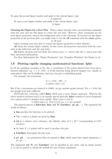
To open the second figure window and make it the current figure, type ≫ figure(2) To open a new figure window and make it the current figure, type ≫ figure Clearing the Figure for a New Plot When a figure already exists, most plotting commands clear the axes and use this figure to create the new plot. However, these commands do not reset figure properties, such as the background color or the colormap. If you have set any figure properties in the previous plot, you might want to use the clf command with the reset option, ≫ clf reset before creating your new plot to restore the figures properties to their defaults. clf clears the current figure window. It also resets all properties associated with the axes, such as the hold state and the axis state. cla deletes all plots and text from the current axes, i.e. leaves only the x- and y-axes and their associated information. For More Information See “Figure Properties” and “Graphics Windows” the Figure in [1]. 1.9 Plotting rapidly changing mathematical functions: fplot In all the graphing examples so far, the x coordinates of the points plotted have been incremented uniformly, e.g. x = 0 : 0.01 : 4. If the function being plotted changes very rapidly in some places, this can be inefficient, and can even give a misleading graph. For example, the statements ≫ x = 0.01 : .001 : .1; ≫ plot(x, sin(1./x)) But if the x increments are reduced to 0.0001, we get another graph instead. For x < 0.04, the two graphs look quite different. MATLAB has a function called fplot which uses a more elegant approach. Whereas the above method evaluates sin(1/x) at equally spaced intervals, fplot evaluates it more frequently over regions where it changes more rapidly. Here’s how to use it: ≫ fplot( sin(1/x), [0.01 0.1])% no, 1./x not needed! The general pattern is fplot(fun, lims, tol, N, ′ LineSpec ′ , pl, p2, . . .). The argument list works as follows. • fun specifies the function to be plotted. • The x and/or y limits are given by lims. • tol is a relative error tolerance, the default value of 2 × 10 −3 corresponding to 0.2% accuracy. • At least N + 1 points will be used to produce the plot. • LineSpec determines the line type. • p1, p2, . . . are parameters that are passed to fun, which must have input arguments x, p1, p2, . . . . The arguments tol, N, and ’LineSpec’ can be specified in any order, and an empty matrix ([ ]) can be passed to obtain the default for any of these arguments. 6
Example 1.6 In this example, fplot produces a graph of the function exp( √ x sin 12x) over the interval 0 ≤ x ≤ 2π. In the second call, we override the default solid line style and specify a dashed line with ′ − − ′ . The argument [0.01 1 − 15 20] in the third call forces limits in both the x and y directions, 0.01 ≤ x ≤ 1 and −15 ≤ y ≤ 20, and ′ − . ′ asks for a dash-dot line style. The final fplot example illustrates how more than one function can be plotted in the same call. subplot(221), fplot( ′ exp(sqrt(x) ∗ sin(12 ∗ x)) ′ , [0 2 ∗ pi]) subplot(222), fplot( ′ sin(round(x)) ′ , [0 10], ′ −− ′ ) subplot(223), fplot( ′ cos(30 ∗ x)/x ′ , [0.01 1 − 15 20], ′ −. ′ ) subplot(224), fplot( ′ [sin(x), cos(2 ∗ x), 1/(1 + x)] ′ , [05 ∗ pi − 1.5 1.5]) Remark 1.3 We remark that: • The two statements plot(x, Y, ′ ms − − ′ ) and plot(x, Y, ′ s − −m ′ ) are equivalent. • You can exert further control by supplying more arguments to plot. The properties LineWidth (default 0.5 points) and MarkerSize (default 6 points) can be specified in points, where a point is 1/72 inch. For example, the commands ≫ plot(x, y, ′ LineWidth ′ , 2) ≫ plot(x, y, ′ p ′ , ′ MarkerSize ′ , 10) produce a plot with a 2-point line width and 10-point marker size, respectively. For markers that have a well-defined interior, the MarkerEdgeColor and MarkerFaceColor can be set to one of the colors in subsection 1.2. So, for example, ≫ plot(x, y, ′ o ′ , ′ Marker Edge Color ′ , ′ m ′ ) gives magenta edges to the circles. ≫ plot(x, y, ′ m − −− ′ , ′ LineWidth ′ , 3, ′ MarkerSize ′ , 5) and the right-hand plot with ≫ plot(x, y, ′ − − rs ′ , ′ MarkerSize ′ , 20, ′ MarkerFaceColor ′ , ′ g ′ ) Default values for these properties, and for some others to be discussed later in the chapter, are summarized in Table 6.1. centerlineTable 6.1. Default values for some properties. LineWidth 0.5 MarkerSize 6 MarkerEdgeColor auto MarkerFaceColor none FontSize 10 FontAngle normal • Using loglog instead of plot causes the axes to be scaled logarithmically. This feature is useful for revealing power-law relationships as straight lines. In the example below we plot |1 + h + h 2 /2 − exp(h)| against h for h = 1, 10 −1 , 10 −2 , 10 −3 , 10 −4 . This quantity behaves like a multiple of h 3 when h is small, and hence on a log-log scale the values should lie close to a straight line of slope 3. To confirm this, we also plot a dashed reference line with the predicted slope, exploiting the fact that more than one set of data can be passed 7
Page 1 and 2: Subjects:: Graphics lecturer in cha
Page 3 and 4: 1.4 Adding Plots to an Existing Gra
Page 5: Example 1.4 The characters \ pi cre
Page 9 and 10: for a = 12 and b = 5. a = 12; b = 5
Page 11 and 12: The matrix a is 30 × 30. The eleme

Matlab Chapter6.pdf

You also want an ePaper? Increase the reach of your titles

Delete template?

Save as template?