Matlab Chapter6.pdf

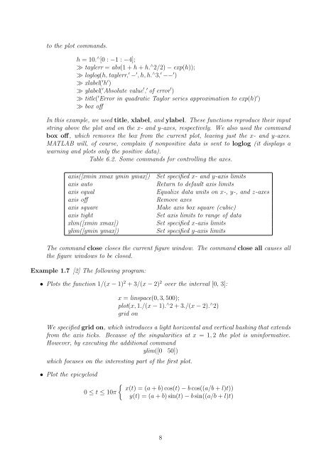
to the plot commands.
h = 10. ∧ [0 : −1 : −4];
≫ taylerr = abs(1 + h + h. ∧ 2/2) − exp(h));
≫ loglog(h, taylerr, ′ − ′ , h, h. ∧ 3, ′ −− ′ )
≫ xlabel( ′ h ′ )
≫ ylabel( ′ Absolute value ′ , ′ of error ′ )
≫ title( ′ Error in quadratic Taylor series approximation to exp(h) ′ )
≫ box off
In this example, we used title, xlabel, and ylabel. These functions reproduce their input
string above the plot and on the x- and y-axes, respectively. We also used the command
box off, which removes the box from the current plot, leaving just the x- and y-axes.
MATLAB will, of course, complain if nonpositive data is sent to loglog (it displays a
warning and plots only the positive data).
Table 6.2. Some commands for controlling the axes.
axis([xmin xmax ymin ymax])
axis auto
axis equal
axis off
axis square
axis tight
xlim([xmin xmax])
ylim([ymin ymax])
Set specified x- and y-axis limits
Return to default axis limits
Equalize data units on x-, y-, and z-axes
Remove axes
Make axis box square (cubic)
Set axis limits to range of data
Set specified x-axis limits
Set specified y-axis limits
The command close closes the current figure window. The command close all causes all
the figure windows to be closed.
Example 1.7 [2] The following program:
• Plots the function 1/(x − 1) 2 + 3/(x − 2) 2 over the interval [0, 3]:
x = linspace(0, 3, 500);
plot(x, 1./(x − 1). ∧ 2 + 3./(x − 2). ∧ 2)
grid on
We specified grid on, which introduces a light horizontal and vertical hashing that extends
from the axis ticks. Because of the singularities at x = 1, 2 the plot is uninformative.
However, by executing the additional command
ylim([0 50])
which focuses on the interesting part of the first plot.
• Plot the epicycloid
0 ≤ t ≤ 10π
{ x(t) = (a + b) cos(t) − b cos((a/b + l)t))
y(t) = (a + b) sin(t) − b sin((a/b + l)t)
8