Matlab Chapter6.pdf

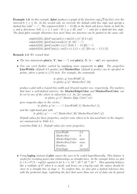
Example 1.6 In this example, fplot produces a graph of the function exp( √ x sin 12x) over the
interval 0 ≤ x ≤ 2π. In the second call, we override the default solid line style and specify a
dashed line with ′ − − ′ . The argument [0.01 1 − 15 20] in the third call forces limits in both the
x and y directions, 0.01 ≤ x ≤ 1 and −15 ≤ y ≤ 20, and ′ − . ′ asks for a dash-dot line style.
The final fplot example illustrates how more than one function can be plotted in the same call.
subplot(221), fplot( ′ exp(sqrt(x) ∗ sin(12 ∗ x)) ′ , [0 2 ∗ pi])
subplot(222), fplot( ′ sin(round(x)) ′ , [0 10], ′ −− ′ )
subplot(223), fplot( ′ cos(30 ∗ x)/x ′ , [0.01 1 − 15 20], ′ −. ′ )
subplot(224), fplot( ′ [sin(x), cos(2 ∗ x), 1/(1 + x)] ′ , [05 ∗ pi − 1.5 1.5])
Remark 1.3 We remark that:
• The two statements plot(x, Y, ′ ms − − ′ ) and plot(x, Y, ′ s − −m ′ ) are equivalent.
• You can exert further control by supplying more arguments to plot. The properties
LineWidth (default 0.5 points) and MarkerSize (default 6 points) can be specified in
points, where a point is 1/72 inch. For example, the commands
≫ plot(x, y, ′ LineWidth ′ , 2)
≫ plot(x, y, ′ p ′ , ′ MarkerSize ′ , 10)
produce a plot with a 2-point line width and 10-point marker size, respectively. For markers
that have a well-defined interior, the MarkerEdgeColor and MarkerFaceColor can
be set to one of the colors in subsection 1.2. So, for example,
≫ plot(x, y, ′ o ′ , ′ Marker Edge Color ′ , ′ m ′ )
gives magenta edges to the circles.
≫ plot(x, y, ′ m − −− ′ , ′ LineWidth ′ , 3, ′ MarkerSize ′ , 5)
and the right-hand plot with
≫ plot(x, y, ′ − − rs ′ , ′ MarkerSize ′ , 20, ′ MarkerFaceColor ′ , ′ g ′ )
Default values for these properties, and for some others to be discussed later in the chapter,
are summarized in Table 6.1.
centerlineTable 6.1. Default values for some properties.
LineWidth 0.5
MarkerSize 6
MarkerEdgeColor auto
MarkerFaceColor none
FontSize 10
FontAngle normal
• Using loglog instead of plot causes the axes to be scaled logarithmically. This feature is
useful for revealing power-law relationships as straight lines. In the example below we plot
|1 + h + h 2 /2 − exp(h)| against h for h = 1, 10 −1 , 10 −2 , 10 −3 , 10 −4 . This quantity behaves
like a multiple of h 3 when h is small, and hence on a log-log scale the values should lie
close to a straight line of slope 3. To confirm this, we also plot a dashed reference line
with the predicted slope, exploiting the fact that more than one set of data can be passed
7