Matlab Chapter6.pdf
Matlab Chapter6.pdf
Matlab Chapter6.pdf

You also want an ePaper? Increase the reach of your titles
YUMPU automatically turns print PDFs into web optimized ePapers that Google loves.
for a = 12 and b = 5.<br />
a = 12; b = 5;<br />
t = 0 : 0.05 : 10 ∗ pi;<br />
x = (a + b) ∗ cos(t) − b ∗ cos(a/b + l) ∗ t);<br />
y = (a + b) ∗ sin(t) − b ∗ sin(a/b + l) ∗ t);<br />
plot(x, y)<br />
axis equal<br />
axis([−25 25 − 25 25])<br />
grid on<br />
title( ′ Epicycloid: a = 12, b = 5 ′ )<br />
xlabel( ′ x(t) ′ ), ylabel( ′ y(t) ′ )<br />
• Plot the Legendre polynomials of degrees 1 to 4 (for the properties of these polynomials,<br />
see, help of matlab) and use the legend function to add a box that explains the line styles.<br />
x = −1 : .01 : 1;<br />
p1 = x;<br />
p2 = (3/2) ∗ x. ∧ 2 − 1/2;<br />
p3 = (5/2) ∗ x. ∧ 3 − (3/2) ∗ x;<br />
p4 = (35/8) ∗ x. ∧ 4 − (15/4) ∗ x. ∧ 2 + 3/8;<br />
plot(x, pl, ′ r : ′ , x, p2, ′ g − − ′ , x, p3, ′ b − . ′ , x, p4, ′ m− ′ )<br />
box off<br />
legend( ′ \it n = 1 ′ , ′ \it n = 2 ′ , ′ \it n = 3 ′ , ′ \it n = 4 ′ , ′ Location ′ , ′ SouthEast ′ )<br />
xlabel( ′ x ′ , ′ FontSize ′ , 12, ′ FontAngle ′ , ′ italic ′ )<br />
ylabel( ′ P n ′ , ′ FontSize ′ , 12, ′ FontAngle ′ , ′ italic ′ , ′ Rotation ′ , 0)<br />
title( ′ Legendre Polynomials ′ , ′ FontSize ′ , 14)<br />
text(−.6, .7, ′ (n + 1)P n + 1(x) = (2n + 1)xP n(x) − nP n − 1(x) ′ , . . .<br />
′ FontSize ′ , 12, ′ FontAngle ′ , ′ italic ′ )<br />
Remark 1.4 Generally, typing legend(’string ′ 1, ’string 2 ’,. . ., ’string n ’) will create a legend<br />
box that puts ’string i ’ next to the color/marker/line style information for the corresponding<br />
plot. By default, the box appears in the top right-hand (northeast) corner of the axis area. The<br />
location of the box can be specified with the syntax legend(’,. . ., ’Location’, location), where<br />
location is a string with possible values that include:<br />
’North’<br />
’NorthWest’<br />
’NorthOutside’<br />
’Best’<br />
’BestOutside’<br />
inside plot box near top<br />
inside top left<br />
outside plot box near top<br />
automatically chosen to give least conflict with data<br />
automatically chosen to leave least unused space outside plot<br />
These values can be abbreviated as ’N’, ’NW ’, etc. In our example we chose the bottom righthand<br />
corner. Once the plot has been drawn, the legend box can be repositioned by putting the<br />
cursor over it and dragging it using the left mouse button. The legend function has many other<br />
options, which can be seen by typing doc legend.<br />
2 3-D plots<br />
MATLAB has a variety of functions for displaying and visualizing data in 3-D, either as lines<br />
in 3-D, or as various types of surfaces. This section provides a brief overview.<br />
9