Design and Analysis of Ultrasonic NDT Instrumentation ... - IJME

——————————————————————————————————————————————–————
The LRUT application uses a 240V pk-pk electrical signal in
the frequency range of 20kHz to 100kHz. The technique
requires a number of excitations (and data collection) at a
repetitive rate (rep-rate) of 0.1s for data manipulation. The
main circuits involved are the transmit-circuit (TX), receive
-circuit (RX), high-voltage power supply (CCPS) and the
digital logic control circuits (DSP). The TX circuit produces
a high-voltage, high-current electrical signal that excites the
transducer array (load) that in turn produces the sound
waves. The receive-circuit allows reception and signal processing
of the echo signals from features. CCPS is a fast
capacitor-charging power supply that produces +/-150V on
demand, which provides voltage to the TX. The DSP handles
system control, signal processing, storage and communication.
Load characterization
Load charecterisation is required for specifying the PRU’s
port dynamics and power performance. Load for the PRU is
an array of PZT transducers of the type EBL#2 [10] that are
pre-engineererd with damping blocks and faceplates. A
number of equivalent circuit models for PZT transducers are
discussed in the literatue [5]. This work employed a singledimensional-thickness
mode Krimholtz, Leedom and
Matthaei (KLM) model, as the KLM model allows
additional layers such as face plates and matching layers to
be easily added on to the model. Faceplates and matching
layers can be modelled using the lossy transmission-line
model. The derivation of parameters used in the KLM model
for the PZT transducer requires three basic parameters
that can only be obtained using practical measurements or
by using equations [11]. They are free capacitance (C T ),
resonant frequency (f p ) and anti-resonant frequency (f a ) of
the transducer. A Solartron SI1260 impedance analyzer was
used for the practical impedance analysis. The measured
free capacitance was approximately 1100pF at an excitation
frequency of 1kHz. The resonant frequency (f p ) and antiresonant
frequency (f a ) were measured as 1.7MHz and
2.4MHz, respectively. Another study claimed that for transducers
having a thickness very much smaller than the other
dimensions, the vibrations in directions other than thickness
are insignificant for modeling purposes [12]. Hence, this
single-dimensional model is adequate for the modeling process
considered here.
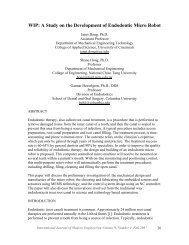
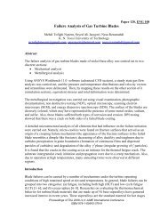
Practical input-impedance analysis results were compared
with the simulation results across the frequency range of
interest. Figure 3 compares the simulation and practical
results obtained for a single PZT. Impedance and phase
graphs are set to show 20% and 2% error bars, respectively.
A good agreement within 20% was obtained between the
simulation and practical results.
Impedance (Ω)
1.00E+04
9.00E+03
8.00E+03
7.00E+03
6.00E+03
5.00E+03
4.00E+03
3.00E+03
2.00E+03
1.00E+03
0.00E+00
1.00E+04
2.00E+04
3.00E+04
Input impedance analysis
(Single ELB#2 transducer)
4.00E+04
5.00E+04
6.00E+04
1.000E+05,
1.699E+03
1.065E+05,
1.369E+03
Figure 3. Input Impedance Analysis of a Single Domain PZT
7.00E+04
In LRUT applications, PZT elements are mounted to
stainless steel backing blocks for damping and mounting
purposes. This transducer fabrication also includes a faceplate
for acoustic impedance matching and durability. The
PZT transducer with backing block and faceplate is called
an LRUT transducer. Each output port in the PRU system is
specified to drive an array of LRUT transducers. The array
size can be as big as 13 LRUT transducers connected in
parallel.
The total input impedance analysis for an array of 13
LRUT transducers was also carried out practically and
through computer simulations. Faceplates were modeled
using a transmission-line model. The stainless steel dampers
were modeled with resisters, whose values were calculated
using the acoustic impedance formula, R =ρAu p , where ρ, A
and u p were the density of stainless steel, cross sectional
area and phase velocity, respectively [13]. The practical and
simulated results are shown in Figure 4. Discrepancies within
30% were observed between practical and simulation
results. As the operating region of the LRUT application
was well below the series resonance frequency of the PZTs,
the load held capacitive properties as expected [11]. This
can be seen in Figure 3, where the phase angles are around
negative 90 degrees (-90°).
A maximum of 40% variation in input capacitance was
observed when practical tests were carried out on two batches
of 77 transducers (within and between the batches).
Hence, the 30% discrepancy observed in Figure 4 was acceptable.
It was concluded from the modeling work that the
minimum value of load impedance was 115Ω±30%
(80.5Ω), which was confirmed through practical results.
8.00E+04
Excitation frequency (kHz)
Impedance - Practical
Phase - Practical
9.00E+04
1.00E+05
1.10E+05
-82
-88
-94
-100
Phase (°)
Impedance - Simulation
Phase - Simulation
——————————————————————————————————————————————–————
90 INTERNATIONAL JOURNAL OF MODERN ENGINEERING | VOLUME 12, NUMBER 1, FALL/WINTER 2011