proofs

A theorem of Pólya on polynomials 141
By Chebyshev’s theorem we deduce
b−a
2 ≥ max |p(x)| ≥ (
a≤x≤b
2 )n 1
2
= 2( b−a
n−1 4 )n ,
and thus b − a ≤ 4, as desired.
This corollary brings us already very close to the statement of Theorem 2.
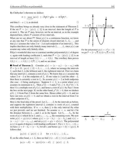
If the set P = {x : |p(x)| ≤ 2} is an interval, then the length of P is
at most 4. The set P may, however, not be an interval, as in the example
depicted here, where P consists of two intervals.
What can we say about P? Since p(x) is a continuous function, we know
at any rate that P is the union of disjoint closed intervals I 1 , I 2 , . . ., and
that p(x) assumes the value 2 or −2 at each endpoint of an interval I j . This
implies that there are only finitely many intervals I 1 , . . . , I t , since p(x) can
assume any value only finitely often.
Pólya’s wonderful idea was to construct another polynomial ˜p(x) of degree
n, again with leading coefficient 1, such that ˜P = {x : |˜p(x)| ≤ 2} is an
interval of length at least l(I 1 ) + . . . + l(I t ). The corollary then proves
l(I 1 ) + . . . + l(I t ) ≤ l( ˜P) ≤ 4, and we are done.
Proof of Theorem 2. Consider p(x) = (x − a 1 ) · · · (x − a n ) with
P = {x ∈ R : |p(x)| ≤ 2} = I 1 ∪ . . . ∪ I t , where we arrange the intervals
I j such that I 1 is the leftmost and I t the rightmost interval. First we claim
that any interval I j contains a root of p(x). We know that p(x) assumes the
values 2 or −2 at the endpoints of I j . If one value is 2 and the other −2,
then there is certainly a root in I j . So assume p(x) = 2 at both endpoints
(the case −2 being analogous). Suppose b ∈ I j is a point where p(x)
assumes its minimum in I j . Then p ′ (b) = 0 and p ′′ (b) ≥ 0. If p ′′ (b) = 0,
then b is a multiple root of p ′ (x), and hence a root of p(x) by Fact 1 from
the box on the next page. If, on the other hand, p ′′ (b) > 0, then we deduce
p(b) ≤ 0 from Fact 2 from the same box. Hence either p(b) = 0, and we
have our root, or p(b) < 0, and we obtain a root in the interval from b to
either endpoint of I j .
Here is the final idea of the proof. Let I 1 , . . .,I t be the intervals as before,
and suppose the rightmost interval I t contains m roots of p(x), counted
with their multiplicities. If m = n, then I t is the only interval (by what
we just proved), and we are finished. So assume m < n, and let d be
the distance between I t−1 and I t as in the figure. Let b 1 , . . . , b m be the
roots of p(x) which lie in I t and c 1 , . . .c n−m the remaining roots. We now
write p(x) = q(x)r(x) where q(x) = (x − b 1 ) · · · (x − b m ) and r(x) =
(x − c 1 ) · · · (x − c n−m ), and set p 1 (x) = q(x + d)r(x). The polynomial
p 1 (x) is again of degree n with leading coefficient 1. For x ∈ I 1 ∪. . .∪I t−1
we have |x + d − b i | < |x − b i | for all i, and hence |q(x + d)| < |q(x)|. It
follows that
|p 1 (x)| ≤ |p(x)| ≤ 2 for x ∈ I 1 ∪ . . . ∪ I t−1 .
If, on the other hand, x ∈ I t , then we find |r(x − d)| ≤ |r(x)| and thus
|p 1 (x − d)| = |q(x)||r(x − d)| ≤ |p(x)| ≤ 2,
□
1− √ 3 1 1+ √ 3 ≈3.20
For the polynomial p(x) = x 2 (x − 3)
we get P = [1− √ 3, 1]∪[1+ √ 3, ≈ 3.2]
I 1
d
. . . { }} {
I
. . .
2 I t−1 I t