- Page 2: Martin Aigner Günter M. Ziegler Pr
- Page 5 and 6: Prof. Dr. Martin Aigner FB Mathemat
- Page 7 and 8: VI Preface to the Fourth Edition Wh
- Page 9 and 10: VIII Table of Contents 21. A theore
- Page 12 and 13: Six proofs of the infinity of prime
- Page 14 and 15: Six proofs of the infinity of prime
- Page 16 and 17: Bertrand’s postulate Chapter 2 We
- Page 18 and 19: Bertrand’s postulate 9 times. Her
- Page 20 and 21: Bertrand’s postulate 11 by compar
- Page 22 and 23: Binomial coefficients are (almost)
- Page 24 and 25: Binomial coefficients are (almost)
- Page 26 and 27: Representing numbers as sums of two
- Page 28 and 29: Representing numbers as sums of two
- Page 30 and 31: Representing numbers as sums of two
- Page 32 and 33: The law of quadratic reciprocity Ch
- Page 34 and 35: The law of quadratic reciprocity 25
- Page 36 and 37: The law of quadratic reciprocity 27
- Page 38 and 39: The law of quadratic reciprocity 29
- Page 40 and 41: Every finite division ring is a fie
- Page 42 and 43: Every finite division ring is a fie
- Page 44 and 45: Some irrational numbers Chapter 7
- Page 46 and 47: Some irrational numbers 37 and this
- Page 48 and 49: Some irrational numbers 39 F(x) may
- Page 50: Some irrational numbers 41 Now assu
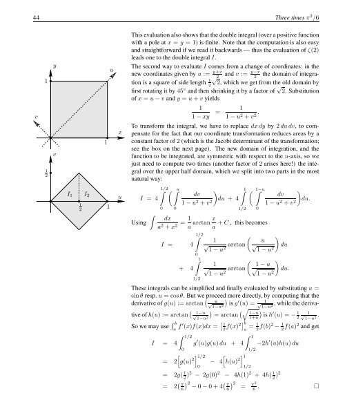
- Page 55 and 56: 46 Three times π 2 /6 For m = 1, 2
- Page 57 and 58: 48 Three times π 2 /6 1 f(t) = 1 t
- Page 59 and 60: 50 Three times π 2 /6 (3) It has b
- Page 62 and 63: Hilbert’s third problem: decompos
- Page 64 and 65: Hilbert’s third problem: decompos
- Page 66 and 67: Hilbert’s third problem: decompos
- Page 68 and 69: Hilbert’s third problem: decompos
- Page 70: Hilbert’s third problem: decompos
- Page 73 and 74: 64 Lines in the plane, and decompos
- Page 75 and 76: 66 Lines in the plane, and decompos
- Page 78 and 79: The slope problem Chapter 11 Try fo
- Page 80 and 81: The slope problem 71 • Every move
- Page 82: The slope problem 73 For the second
- Page 85 and 86: 76 Three applications of Euler’s
- Page 87 and 88: 78 Three applications of Euler’s
- Page 89 and 90: 80 Three applications of Euler’s
- Page 91 and 92: 82 Cauchy’s rigidity theorem Q: Q
- Page 93 and 94: 84 Cauchy’s rigidity theorem A be
- Page 95 and 96: 86 Touching simplices l l l ′ Pr
- Page 97 and 98: 88 Touching simplices For our examp
- Page 99 and 100: 90 Every large point set has an obt
- Page 101 and 102:
92 Every large point set has an obt
- Page 103 and 104:
94 Every large point set has an obt
- Page 105 and 106:
96 Borsuk’s conjecture Theorem. L
- Page 107 and 108:
98 Borsuk’s conjecture On the oth
- Page 109 and 110:
100 Borsuk’s conjecture To obtain
- Page 112 and 113:
Sets, functions, and the continuum
- Page 114 and 115:
Sets, functions, and the continuum
- Page 116 and 117:
Sets, functions, and the continuum
- Page 118 and 119:
Sets, functions, and the continuum
- Page 120 and 121:
Sets, functions, and the continuum
- Page 122 and 123:
Sets, functions, and the continuum
- Page 124 and 125:
Sets, functions, and the continuum
- Page 126 and 127:
Sets, functions, and the continuum
- Page 128 and 129:
In praise of inequalities Chapter 1
- Page 130 and 131:
In praise of inequalities 121 where
- Page 132 and 133:
In praise of inequalities 123 Proo
- Page 134:
In praise of inequalities 125 Seco
- Page 137 and 138:
128 The fundamental theorem of alge
- Page 140 and 141:
One square and an odd number of tri
- Page 142 and 143:
One square and an odd number of tri
- Page 144 and 145:
One square and an odd number of tri
- Page 146 and 147:
One square and an odd number of tri
- Page 148 and 149:
A theorem of Pólya on polynomials
- Page 150 and 151:
A theorem of Pólya on polynomials
- Page 152 and 153:
A theorem of Pólya on polynomials
- Page 154 and 155:
On a lemma of Littlewood and Offord
- Page 156 and 157:
On a lemma of Littlewood and Offord
- Page 158 and 159:
Cotangent and the Herglotz trick Ch
- Page 160 and 161:
Cotangent and the Herglotz trick 15
- Page 162 and 163:
Cotangent and the Herglotz trick 15
- Page 164 and 165:
Buffon’s needle problem Chapter 2
- Page 166 and 167:
Buffon’s needle problem 157 The c
- Page 168:
Combinatorics 25 Pigeon-hole and do
- Page 171 and 172:
162 Pigeon-hole and double counting
- Page 173 and 174:
164 Pigeon-hole and double counting
- Page 175 and 176:
166 Pigeon-hole and double counting
- Page 177 and 178:
168 Pigeon-hole and double counting
- Page 179 and 180:
170 Pigeon-hole and double counting
- Page 182 and 183:
Tiling rectangles Chapter 26 Some m
- Page 184 and 185:
Tiling rectangles 175 Third proof.
- Page 186:
Tiling rectangles 177 References [1
- Page 189 and 190:
180 Three famous theorems on finite
- Page 191 and 192:
182 Three famous theorems on finite
- Page 194 and 195:
Shuffling cards Chapter 28 How ofte
- Page 196 and 197:
Shuffling cards 187 Indeed, if A i
- Page 198 and 199:
Shuffling cards 189 Let T be the nu
- Page 200 and 201:
Shuffling cards 191 Theorem 1. Let
- Page 202 and 203:
Shuffling cards 193 Proof. (1) We
- Page 204 and 205:
Lattice paths and determinants Chap
- Page 206 and 207:
Lattice paths and determinants 197
- Page 208 and 209:
Lattice paths and determinants 199
- Page 210 and 211:
Cayley’s formula for the number o
- Page 212 and 213:
Cayley’s formula for the number o
- Page 214 and 215:
Cayley’s formula for the number o
- Page 216 and 217:
Identities versus bijections Chapte
- Page 218 and 219:
Identities versus bijections 209 Pr
- Page 220 and 221:
Identities versus bijections 211 As
- Page 222 and 223:
Completing Latin squares Chapter 32
- Page 224 and 225:
Completing Latin squares 215 Proof
- Page 226 and 227:
Completing Latin squares 217 be dis
- Page 228:
Graph Theory 33 The Dinitz problem
- Page 231 and 232:
222 The Dinitz problem In 1976 Vizi
- Page 233 and 234:
224 The Dinitz problem X A bipartit
- Page 235 and 236:
226 The Dinitz problem G : L(G) : a
- Page 237 and 238:
228 Five-coloring plane graphs From
- Page 239 and 240:
230 Five-coloring plane graphs is s
- Page 241 and 242:
232 How to guard a museum The follo
- Page 243 and 244:
234 How to guard a museum “Museum
- Page 245 and 246:
236 Turán’s graph theorem Let us
- Page 247 and 248:
238 Turán’s graph theorem Thus b
- Page 250 and 251:
Communicating without errors Chapte
- Page 252 and 253:
Communicating without errors 243 cl
- Page 254 and 255:
Communicating without errors 245 Le
- Page 256 and 257:
Communicating without errors 247 On
- Page 258 and 259:
Communicating without errors 249 No
- Page 260 and 261:
The chromatic number of Kneser grap
- Page 262 and 263:
The chromatic number of Kneser grap
- Page 264:
The chromatic number of Kneser grap
- Page 267 and 268:
258 Of friends and politicians w 1
- Page 270 and 271:
Probability makes counting (sometim
- Page 272 and 273:
Probability makes counting (sometim
- Page 274 and 275:
Probability makes counting (sometim
- Page 276 and 277:
Probability makes counting (sometim
- Page 278 and 279:
Proofs from THE BOOK 269
- Page 280 and 281:
Index acyclic directed graph, 196 a
- Page 282 and 283:
Index 273 matrix-tree theorem, 203