Undrained Load Capacity of Torpedo Anchors in ... - laceo - UFRJ

Proceedings of the ASME 2009 28th International Conference on Ocean, Offshore and Arctic Engineering
OMAE2009
May 31 - June 5, 2009, Honolulu, Hawaii, USA
Proceedings of the ASME 28th International Conference on Ocean, Offshore and Arctic Engineering
OMAE2009
May 31 – June 5, 2009, Honolulu, Hawaii
OMAE2009-79465
OMAE2009-79465
UNDRAINED LOAD CAPACITY OF TORPEDO ANCHORS IN COHESIVE SOILS
Cristiano S. de Aguiar
COPPE/UFRJ
Rio de Janeiro, Brazil
José Renato M. de Sousa
COPPE/UFRJ
Rio de Janeiro, Brazil
Gilberto Bruno Ellwanger
COPPE/UFRJ
Rio de Janeiro, Brazil
Elisabeth de Campos Porto
PETROBRAS
Rio de Janeiro, Brazil
Cipriano José de M. Júnior
PETROBRAS
Rio de Janeiro, Brazil
Diego Foppa
PETROBRAS
Rio de Janeiro, Brazil
ABSTRACT
This paper presents a numerical based study on the
undrained load capacity of a typical torpedo anchor embedded
in a purely cohesive isotropic soil using a three-dimensional
nonlinear finite element (FE) model. In this model, the soil is
simulated with solid elements capable of representing its
nonlinear physical behavior as well as the large deformations
involved. The torpedo anchor is also modeled with solid
elements and its complex geometry is represented. Moreover,
the anchor-soil interaction is addressed with contact finite
elements that allow relative sliding with friction between the
surfaces in contact. Various analyses are conducted in order to
understand the response of this type of anchor when different
soil undrained shear strengths, load directions as well as
number and width of flukes are considered. The obtained
results point to two different failure mechanisms: one that
mobilizes a great amount of soil and is directly related to its
lateral resistance; and a second one that mobilizes a small
amount of soil and is related to the vertical resistance of the
soil. Besides, the total contact area of the anchor seems to be an
important parameter in the determination of its load capacity
and, consequently, the increase of the undrained shear strength
and the number of flukes and/or their width significantly
increases the load capacity of the anchor.
INTRODUCTION
As a consequence of the great global demand for oil and
gas, the offshore exploitation frontier is moving fast to water
depths around 3000m. Moreover, the high number of floating
production and drilling units in operation may provoke the
congestion of the sea bottom due to the high number of risers
and mooring lines employed. Hence, the development of
optimized mooring systems demands lower mooring radius and
low cost anchors designed to hold high loads. In this scenario,
the torpedo anchor has been proven to be an outstanding
alternative in Brazilian offshore fields.
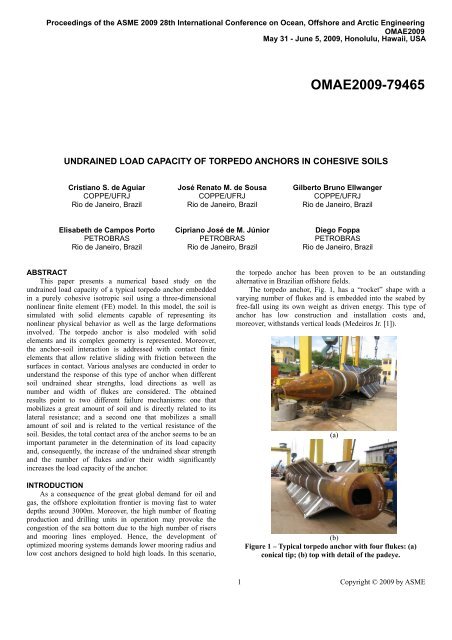
The torpedo anchor, Fig. 1, has a “rocket” shape with a
varying number of flukes and is embedded into the seabed by
free-fall using its own weight as driven energy. This type of
anchor has low construction and installation costs and,
moreover, withstands vertical loads (Medeiros Jr. [1]).
(a)
(b)
Figure 1 – Typical torpedo anchor with four flukes: (a)
conical tip; (b) top with detail of the padeye.
1 Copyright © 2009 by ASME

Torpedo anchors were first employed to hold flexible risers where [ Δσ] = [ Δσ
] T
xx Δσ
yy Δσ
zz Δτ
xy Δτ
xz Δτ
yz is the
just after their touchdown points (TDP) in order to avoid that
the loads generated by the floating units movements were
incremental total stress vector;
transferred to subsea equipments such as wet Christmas trees [ Δε
] = [ Δε
] T
xx Δε
yy Δε
zz Δγ
xy Δγ
xz Δγ
yz is the incremental
(Medeiros Jr. [1]). In 2003, a high holding capacity torpedo total strain vector; and [ D
ep
] is the constitutive elasto-plastic
anchor was designed to sustain the loads imposed by the
matrix (Potts and Zdravkovic [4]):
mooring lines of Petrobras FPSO P-50 (Araújo et al. [2]). Since
E
[ Δσ] [ Dep ] [ Δε]
K s =
3⋅
1−
2⋅υ
(6)
then, other floating production systems have been anchored
T
using the torpedo concept (Brandão et al. [3]).
⎧∂P
[ ]
([ σ] ,[ m]
) ⎫ ⎧∂F( [ σ][ , k]
) ⎫
D ⋅ ⎨ ⎬ ⋅ ⎨ ⎬ ⋅ [ D]
Despite its large use in Brazilian offshore applications, the
[
calculus of the torpedo anchor load capacity and the prediction
] [ ]
⎩ ∂σ
⎭ ⎩ ∂σ
= D −
⎭
T
⎧∂F( [ σ][ , k]
) ⎫ ⎧∂P
of the stresses in its structure due to the loads imposed by the
[ ]
([ σ][ m]
) ⎫
⎨ ⎬ ⋅ D ⋅ ⎨
⎬
⎩ ∂σ
⎭ ⎩ ∂σ
⎭
attached mooring line remains as a great challenge. Thus,
(2)
aiming at accomplishing these tasks, a nonlinear threedimensional
finite element (FE) model is here proposed. This
where [ D ] is the elastic total stress constitutive matrix;
model employs isoparametric solid elements to represent both P ([ σ ],
[ m]
) is the plastic potential function; F ([ σ ],
[ k]
) is the
the soil and the anchor. These elements are capable of yield function; [ σ ] is the stress state in the element; [ m ] and
representing the physical nonlinear behavior of the soil and, [ k ] are state parameters related to the plastic potential and yield
eventually, of the anchor. Large deformations may also be
functions, respectively.
accounted for. Soil-anchor interaction is assured by surface to
The elastic total stress constitutive matrix can be split in
surface contact elements placed on the external surface of the
two parts, as follows:
anchor and the surrounding soil. A general overview of this
model is presented in Fig. 2.
[ D ] = [ D eff ] + [ D pore ]
(3)
where [ D
eff
] is the effective stress constitutive matrix and
[ D
pore
] is the pore fluid stiffness, which, considering an
isotropic material loaded under undrained conditions, are given
by (Zdravkovic and Potts [4]):
⎡ 4 2 2
⎤
⎢K
s + ⋅G
K s − ⋅G
K s − ⋅G
0 0 0
3 3 3
⎥
⎢
4 2
⎥
⎢
K
⎥
s + ⋅G
K s − ⋅G
0 0 0
⎢
3 3
⎥
[ D ] = ⎢
4
⎥
eff
⎢
K s + ⋅G
0 0 0
3
⎥
⎢
symmetric
G 0 0 ⎥
⎢
⎥
⎢
G 0 ⎥
Figure 2 – General view of the FE model.
⎢
⎥
⎣
G⎦
(4)
In this paper, a parametric study is conducted considering a
typical torpedo anchor embedded in a purely cohesive isotropic
⎡1
1 1 0 0 0⎤
soil. The effects on the holding capacity of the undrained soil
⎢
⎥
strength, the number of flukes in the anchor and the width of
⎢
1 1 1 0 0 0
⎥
⎢1
1 1 0 0 0⎥
these flukes are evaluated.
[ D pore ] = K pore ⋅ ⎢
⎥
(5)
⎢0
0 0 0 0 0⎥
⎢
⎥
FE MODEL
0 0 0 0 0 0
⎢
⎥
⎢⎣
0 0 0 0 0 0⎥⎦
Soil modeling
where K
s
is the bulk modulus of the soil, G is the effective
Constitutive matrix
The soil is assumed to be a perfectly elasto-plastic isotropic transverse modulus of the soil and K
pore
is the bulk modulus of
material with physical properties variable with depth. Hence, the fluid, which are given by:
the relation between stresses and strains is given in the form:
( )
2 Copyright © 2009 by ASME

E
G =
(7)
2⋅
K
( 1+υ)
= 1000 ⋅
(8)
pore K s
in which E and υ are the soil effective elastic modulus and
Poisson coefficient, respectively.
In order to represent the nonlinear material behavior of the
soil, the Drucker-Prager model was chosen. This model
approximates the irregular hexagon of the Mohr-Coulomb
failure surface by a circle and, consequently, the Drucker-
Prager yield function is a cylindrical cone as pointed out in Fig.
3.
Figure 3 – Drucker-Prager yield surface in principal stress
space (Potts and Zdravkovic [4]).
The yield function and plastic potential function for this
model are given by (Chen and Baladi [5]):
([ ][ ]) () 1 (2)
k = J + k ⋅ I k
F σ +
(9)
, 2 DP 1 DP
([ ][ ]) () 1
(2)
m = J + m ⋅ I m
P σ +
(10)
, 2 DP 1 DP
where I 1 and J 2 are, respectively, the first and the second
invariant of the stress tensor; k () 1 DP , ( 2
k
)
DP , () 1
m DP and ( 2
m
)
DP are
stress state parameters. These parameters depend on the
adopted approximation to the Mohr-Coulomb hexagon and are
functions of the internal friction angle, φ, the dilation angle, ψ,
and the cohesion, c, of the soil. Figure 4 presents three possible
approximations and Table 1 presents the values of the
parameters for each case:
1. The circle circumscribes the hexagon defined by the
Mohr-Coulomb criterion and passes through the points
of maximum tension (extension circle).
2. The circle circumscribes the hexagon defined by the
Mohr-Coulomb criteria and passes through the points
of maximum compression (compression circle).
3. The circle inscribes the hexagon defined by the Mohr-
Coulomb criteria.
Figure 4 – Drucker-Prager and Mohr-Coulomb yield
surfaces in the deviatoric plane (Potts and Zdravkovic [4]).
1
2
3
Table 1 – Drucker-Prager parameters for different
approximations.
k
( 1 )
() 1
m
( 2) ( 2
k =
)
3 ⋅
DP
DP
DP m DP
⋅ sen( φ)
[ 3 + sen( φ)
]
2 ⋅ sen( ψ )
3 ⋅[ 3 + sen( ψ )]
6 ⋅ c ⋅ cos( φ)
3 ⋅[ 3 + sen( φ)
]
⋅ sen( φ)
2 ⋅ sen( ψ ) 6 ⋅ c ⋅ cos( φ)
[ 3 − sen( φ)
] 3 ⋅[ 3 − sen( ψ )]
3 ⋅[ 3 − sen( φ)
]
sen( φ)
sen( ψ )
3⋅ c cos( φ)
2
3 + sen ( φ)
3 ⋅
2
3 + sen ( ψ ) 3 ⋅
2
3 + sen ( φ)
2
2
3 ⋅
3 ⋅
NOTES:
1: Extension cone (circumscribed).
2: Compression cone (circumscribed).
3: Inscribed cone.
As the model is devoted to the analysis of torpedo anchors
in undrained conditions, the undrained shear strength of the
soil, S u , may replace the cohesion, c, in the expressions
presented in Table 1.
Finally, since the elastic constitutive matrix, Eqs. (3) to (8),
the yield and plastic potential functions, Eqs. (9) and (10), are
determined, the elasto-plastic constitutive matrix is established.
A particular case of the proposed model occurs when the
soil is assumed to be purely cohesive, i. e., φ = 0°. In this case,
the Drucker-Prager yield function, Eq. (9) reduces to:
(2)
([ ] [ k]
) = J k
σ (11)
F , 2 + DP
where, for the circumscribed cylindrical cone approximation,
(2) 2
( 2)
kDP = ⋅ S u and for the inscribed cylindrical cone kDP
= ⋅Su
.
3
The Huber-Von Mises yield function is given by (Chen and
Baladi [5]):
([ ], [ k]
) = J2
kVM
F σ +
(12)
3 Copyright © 2009 by ASME

where:
σ y
k VM = (13)
3
torpedo anchor, H p , the length of the anchor, H e , and the
distance of the tip of the torpedo anchor to the bottom of the FE
mesh, H a .
and σ y is the yield or failure stress of the material.
(2)
In Eqs. (11) and (12), if k VM
are made equal to k
DP , the
Drucker-Prager yield function is equivalent to the Huber-Von
Mises yield function. This leads to equivalent failure stresses,
σ
y
, equal to:
• For the circumscribed cylindrical cone approximation:
σ y = 2 ⋅ S u
(14)
• For the inscribed cylindrical cone approximation:
σ y = 3 ⋅ S u
(15)
Another relevant aspect is that the coefficient of lateral
earth pressure, K 0 , which is the ratio between the vertical and
horizontal effective stress, is related to the internal friction
angle by the relation:
( )
K 0 = 1−
sin φ
(16)
If the soil is assumed to be purely cohesive, the coefficient
of lateral earth pressure is equal to 1,0. However, the Poisson
coefficient can be expressed as:
K0
υ =
(17)
1+
K
0
If K 0 is equal to 1,0, Eq. (16) points to a Poisson coefficient
of 0,5, which leads to numerical problems in the effective stress
constitutive matrix, Eq. (4), since all terms become infinite. In
this case, Potts and Zdravkovic [4] suggest that the Poisson
coefficient should be less than 0,490 and not equal to 0,500. In
this work, a value of 0,495 is chosen whenever this situation
occurs.
Furthermore, as the Poisson coefficient is close to 0,500,
the material is said to be nearly incompressible and volumetric
locking may occur in the FE mesh. To avoid such problem, the
numerical integration of each soil element is performed with
the enhanced strain method.
FE mesh characteristics
As pointed out before, the soil is modeled with hexahedral
and prismatic isoparametric solid elements. These elements
have eight nodes and each node has three degrees of freedom:
translations in directions X, Y and Z. An overview of the main
dimensions of the soil mesh is shown in Fig. 5. The proposed
mesh is a cylinder with a base diameter of 20D, where D is the
diameter of the torpedo anchor including its flukes. The height
of the cylinder is given by the sum of the penetration of the
Figure 5 – Main dimensions of the soil mesh.
Each “slice” of the cylinder has its own physical properties
and, consequently, variable strength, density, longitudinal and
transverse moduli and Poisson coefficients may be assumed.
Each element corresponds to 1/10 of the circumference and
has the other dimensions varying between 10cm to 25cm in the
regions where high plastic strains are expected to occur (close
to the anchor) and between 25cm and 50cm in regions far from
the anchor, as shown in Fig. 5.
These dimensions were adopted after a set of analysis had
been performed. In these analyses, three different mesh
densities (dense, intermediate and coarse) were considered. All
of them were similar in topology. The coarse mesh has about
half the elements used in the intermediate mesh, while the
number of elements in the dense mesh is the double employed
in the intermediate mesh. As the intermediate and dense meshes
did not present significant differences, concerning the
displacements magnitude, the intermediate one was adopted in
this work.
The vertical displacement of the cylinder is restrained at
the nodes of its base. The nodes of its outer wall have their
displacements in X and Z directions restrained and, when a
plane of symmetry is found, the out of plane displacements are
also restrained. In order to avoid a possible influence of these
boundary conditions on the response of the anchor, several
mesh tests were performed. In these tests, the cylinder diameter
and the distance from the tip of the anchor to the bottom of the
mesh (H a ) were varied. It was observed that a diameter of 20D
for the cylinder and a distance of 5,0m for H a were enough to
simulate an “infinite” media.
4 Copyright © 2009 by ASME

Anchor modeling
The torpedo anchor is modeled with eight node
isoparametric solid elements analogous to the ones used in soil
representation. These elements, as pointed out before, are
capable of considering both material and geometrical
nonlinearities. A typical FE mesh of a torpedo anchor is pointed
out in Fig. 6.
Anchor-soil interaction
Figure 7 – Load application.
(a)
(b)
Figure 6 – General view of a FE mesh for a torpedo anchor:
(a) top; and (b) bottom part of the flukes.
A typical FE mesh for a torpedo anchor is more refined at
its top and at the bottom of the flukes, where stress
concentration is expected to occur. In these regions, the
maximum admissible lengths for the elements are forced to be
5,0cm x 9,0cm (height x width) with two divisions along the
thickness of the flukes and tube.
In order to properly represent the bending of the flukes and
the tube and, consequently, avoid shear locking problems, the
numerical integration of each element is performed with the
enhanced strain method.
It is worth mentioning that neither the padeye at the top of
the anchor nor the mooring line are represented in the proposed
model. Hence, the load from the mooring line is applied at the
gravity center of the padeye, where a node is placed and rigidly
connected to the top of the anchor by rigid bars, as presented in
Fig. 7.
Contact assumptions
In problems involving contact between two boundaries,
one of them is usually defined to be the “target” surface, and
the other is the “contact” surface. These two surfaces together
comprise the surface to surface contact pair. “Target” and
“contact” elements that make up a contact pair are associated
with each other via common physical properties, which are
described later.
The “contact” surface are constrained against penetrating
the “target” surface and, usually, the “contact” surface is
defined to be the softer between the two. In the proposed
model, as the anchor is much stiffer than the surrounding soil,
an asymmetric contact approach is chosen and all “target”
elements are placed on the outer wall of the anchor and all
“contact” elements are on the surrounding soil contact surface.
As soil properties vary with depth, so do the contact
properties and, consequently, multiple sets of contact pairs need
to be defined. Therefore, here, each soil surface in contact with
the anchor has contact elements with different physical
properties.
Another important aspect is that surface to surface contact
elements allow large relative displacement and
contact/separation between two surfaces. When a lateral load is
imposed to the anchor, the possible separation between the
anchor and the soil and the consequent formation of a crack
behind the anchor as it moves forward is referred in practice as
“gapping”. According to Potts and Zdravkovic [6], this
phenomenon depends on the soil strength and on its distribution
with depth. For lightly overconsolidated clays, such as the ones
found in Campos Basin, whether gapping occurs or not seem to
not affect the response of piles. Therefore, the developed model
initially assumes that the lateral and top faces of the flukes and,
furthermore, the top and the outer wall of the tube cannot
separate from the surrounding soil, but relative sliding is
allowed. Nevertheless, the conical tip and the bottom of the
flukes are allowed to separate from the soil and possible suction
vertical forces are not accounted by the model.
5 Copyright © 2009 by ASME

Contact properties
As pointed out before, surface to surface contact elements
allow large relative displacement and separation between
surfaces in contact. This task is performed with a contact
detection algorithm based on the pinball technique (Belytschko
and Neal [7]) and contact forces evaluated with the augmented
Lagrangian method (Belytschko et al. [8]).
The augmented Lagrangian method consists of calculating
a series of penalty forces during the equilibrium iterations so
that the final penetration between the two contact bodies is
smaller than a value previously established. In the developed
model, an allowable penetration of 0.1% of the smaller
thickness between the two elements initially in contact is
adopted.
Penalty forces are calculated by placing fictitious springs
along the contact boundaries of two bodies. When contact is
established, these forces are applied to the nodal points of the
contact elements placed along the contact bodies. The forces
are proportional to the penetration and a chosen penalty
parameter, which can be physically interpreted as the stiffness
of the springs.
The choice of the stiffness of the springs, called normal
contact stiffness, f N , may be performed with relatively
simplicity, but respecting some rules. On the one hand, very
high values may lead to numerical instabilities and, on the other
hand, very small values provoke violations of the contact
conditions. Different estimates of contact normal stiffness
proposed in Belytschko and Neal [7] and Benson and Hallquist
[9], for instance, points to a value equivalent to the stiffness of
the elements in contact. Therefore, an estimate of the normal
contact stiffness may be given by:
E(
z)
fN
z)
= ⋅ Ac
tc
( (18)
where t c is the smaller thickness of the two elements in contact
and A c is the contact area between these elements.
Another important aspect is the simulation of the relative
sliding between the soil and the torpedo anchor. Here, the
Mohr-Coulomb friction model is used and, according to API
[10] may be expressed in the form:
−0.5
() z , ψ () z
−0.25
() z , ψ () z
⎪
⎧0.5
⋅ψ
≤ 1.0
α () z = ⎨
(21)
⎪⎩ 0.5 ⋅ψ
> 1.0
where:
( z)
() z
Su
ψ () z =
(22)
p
o
Finally, a stick stiffness, f T , must be defined to avoid large
displacements between the two contact surfaces before the
maximum shear stress is reached. In the proposed model, an
expression similar to the one employed to the normal contact
stiffness was adopted:
G(
z)
fT
( z)
= ⋅ Ac
(23)
t
c
If a purely cohesive soil is modeled, Eq. (9) reduces to:
( z) = α( z) ⋅ S ( z)
τ (24)
max
u
and only this initial adhesion is considered by the contact
elements.
Initial stress state of the soil
An important aspect of the anchor analysis is the
simulation of the initial stress state of the soil, i. e., the stresses
in the soil prior to the imposition of any kind of structural load
to the anchor. As the proposed FE model does not simulate the
anchor penetration in the soil, it is assumed, by hypothesis, that
the anchor is loaded with the soil stress state undisturbed by the
installation process. The anchor, thus, is supposed to be
“wished in place”.
In order to induce this undisturbed stress state in the soil,
three different FE meshes are present in the same FE model: the
first mesh represents the soil that surrounds the anchor; the
second is related to the torpedo anchor; and the third simulates
the soil that occupies the anchor position before its installation.
Figure 8 presents these meshes.
τ
max
( z) = α( z) ⋅ S ( z) + K ( z) ⋅ p ( z) tan( δ )
u
0 0 ⋅
(19)
where τ max is the maximum allowable shear stress; α is the
adhesion factor; p o is the effective overburden pressure; and
δ is the friction angle between the soil and the anchor wall and
may be stated as (API [10]):
o
δ = φ − 5
(20)
The adhesion factor may be calculated by the formulas
proposed by API [10]:
Figure 8 – FE meshes for the analysis of a torpedo anchor:
soil mesh, anchor mesh and soil mesh previous to the
anchor installation.
6 Copyright © 2009 by ASME

The FE mesh of the anchor interacts with the surrounding
soil with the contact elements previously described, as pointed
in Fig. 9(a). The FE mesh of the soil that is at the same position
of the anchor has the shape of the anchor and its outer nodes are
coincident with the surrounding soil nodes. These nodes have
their degrees of freedom coupled, as shown in Fig. 9(b).
Moreover, each “slice” of the meshes presented in Fig. 9(b) has
the same physical properties and, consequently, this mesh
represents the media before the anchor installation. It is
important to mention that there is no interaction between the
meshes of the anchor or the soil that occupies its position.
(a)
(b)
Figure 9 – Details of the FE mesh: (a) surrounding soil and
torpedo anchor; (b) surrounding soil and soil within the
torpedo anchor location.
With this approach, in a first step, the anchor mesh is
“deactivated” by multiplying the stiffness matrix of each of its
elements by a small factor, e. g., 10 -6 , while the remaining soil
finite elements maintain their stiffness matrices. In this step,
only gravity acts and effective material properties are
considered. Therefore, the soil mesh is deformed by its selfweight
and the initial stress state of the soil is defined. The
normal contact forces between the surrounding soil mesh and
the soil mesh at the anchor position are transmitted to the
contact elements that connect the surrounding soil mesh and the
deactivated anchor mesh. In a second load step, the soil at the
anchor position is deactivated and the anchor mesh is activated.
The contact forces are transmitted to the anchor outer wall by
the contact elements and friction forces, as defined in the
previous section, arise when the anchor is loaded.
If the self-weight of the anchor is to be addressed in the
analysis, previous to the application of the load imposed by the
mooring line, a load step in which only gravity acts on the
anchor is included. By doing this, a small perturbation in the
stress state of the soil is induced in the region around the
anchor, which can be argued to be caused by the installation
process.
Solution procedure
A typical FE mesh to predict the load capacity and the
structural behavior of a torpedo anchor has between 100000
and 500000 degrees of freedom and, as previously mentioned,
must account for contact, geometric and material nonlinearities.
After testing several numerical methods, the sparse method was
adopted since it provided accurate results with minimal
computational effort.
The analysis is divided in three different steps. In the first
one, the initial stress state is generated by subjecting the soil to
the action of gravity in a single load increment. In the second
step, the analysis is restarted with the stress state from the first
step and gravity acts on the anchor. This second load step is
also performed with a single load increment. Finally, in the
third step, the total load is imposed with adaptable increments
since, as the surrounding soil progressively fails, the stability of
the solution is affected and lower load increments are required.
Typically, this last load step starts with an initial load increment
of 5% of the total load applied and, as the analysis progresses,
it can be reduced to 1% of the total load.
At each load step, convergence is achieved if the Euclidian
norm (L2) of the residual forces and moments is less than 0.1%
of the absolute value of the total forces and moments applied.
Model implementation
The presented model was implemented in a program called
ESTACAS. This software generates FE meshes to be analyzed
with ANSYS® program, where the following finite elements
are employed: SOLID185 in order to model the soil and the
torpedo anchor; CONTA174 and TARGE170 are used to
simulate the contact between the soil and the anchor.
CASE STUDY
Description
In this paper, various FE analyses were performed in order
to study the effect of four parameters on the hold capacity of
the anchor. These parameters are the:
1. Undrained shear strength of the soil.
2. Number of flukes in the anchor.
3. Width of the flukes.
4. Angle between the applied load and the plane of the
flukes.
The geometry of the anchor is presented in Fig. 10 and its
possible cross-sections are shown in Fig. 11. Initially, the
anchor is assumed to have four flukes, but configurations with
three or no flukes are also studied. The width of the flukes
7 Copyright © 2009 by ASME

varies from 0 to 0.90m. The self-weight of the anchor was kept
constant and equals to 850kN.
Although the undrained shear strengths were different, all
the scenarios have the same anchor penetration. A study based
on the theoretical model presented by True [11] was conducted
only for soil B and the four flukes anchor. The penetration
achieved by the top of the anchor was equal to 16m and this
value was used in all analyses.
Moreover, in the performed analyses, the extension cone
approximation, Eq.(14), is employed.
Several FE meshes were developed. In average, they have
53770 nodes, 93830 elements leading to a problem with
161310 degrees of freedom.
Results
Figure 10 – Dimensions, in m, of the analyzed torpedo
anchor.
Effect of different undrained shear strengths
Figures 12 to 14 present the variation of the displacement
at the top of the anchor with the applied load. These curves
were obtained in the analyses of the torpedo anchor with 4
flukes embedded in soils A, B and C, respectively. In these
figures, loads are at an angle of 45° with the plane of the flukes
(plane 1, Fig. 11a) and several different load inclinations with
respect to the horizontal plane are accounted.
These figures point that the ratio between the displacement
change and the applied load varies with the load inclination
and, consequently, there is a significant difference between the
vertical and lateral soil stiffness.
7000
6000
Figure 11 – Torpedo anchor cross-sections: (a) four, (b)
three and (c) no flukes.
In all analyses, seven load inclinations with respect to the
horizontal plane were considered: 0° (horizontal load), 15°,
30°, 45°, 60°, 75° and 90° (vertical load). All loads, F a , were
applied at the top of the anchor, as pointed out in Fig. 10.
The soil is considered to be purely cohesive and isotropic
with Young modulus varying with depth and given by the
expression:
() z
E( z)
= 550⋅ S
(25)
u
Three different undrained shear strength profiles were
considered in this numerical-based study:
kPa
Soil A: S u ( z)
= 1.5⋅
⋅ z
m
kPa
Soil B: S u ( z)
= 3.0 ⋅ ⋅ z
m
kPa
Soil C: S u ( z)
= 6.0 ⋅ ⋅ z
m
where z is the depth bellow mudline in m.
(26)
Load (kN)
5000
4000
3000
0°
15°
2000
30°
45°
60°
1000
75°
90°
0
0.00 0.05 0.10 0.15 0.20 0.25
Displacement at anchor top (m)
Figure 12 – Load vs displacement curves of a torpedo
anchor with 4 flukes considering different load inclinations
with the horizontal plane: soil A, 45° with the flukes.
8 Copyright © 2009 by ASME

Load (kN)
14000
12000
10000
8000
6000
4000
2000
0
0.00 0.05 0.10 0.15 0.20 0.25 0.30
Displacement at anchor top (m)
0°
15°
30°
45°
60°
75°
90°
Figure 13 – Load vs displacement curves of a torpedo
anchor with 4 flukes considering different load inclinations
with the horizontal plane: soil B, 45° with the flukes.
In order to better understand the failure mechanism of the
soil, Fig. 15 presents its stress state ratio in the last load step of
the analyses performed with soil B. The stress state ratio is
defined to be the ratio between the stress at a point and its yield
or failure stress. When the failure stress is reached, the ratio is
equal to 1. Stress state ratio distributions analogous to the ones
presented in Fig. 15 are also observed in the analyses of soils A
and C.
(a) (b) (c)
25000
20000
Load (kN)
15000
10000
0°
15°
30°
5000
45°
60°
75°
90°
0
0.00 0.05 0.10 0.15 0.20 0.25 0.30
Displacement at anchor top (m)
Figure 14 – Load vs displacement curves of a torpedo
anchor with 4 flukes considering different load inclinations
towards the horizontal plane: soil C, 45° with the flukes.
Moreover, for load inclinations greater than 45°, the failure
of the soil is clear, as the total displacement rapidly grows with
a small change in the applied load. However, for lower
inclinations, there is not a clear sign of failure, but the ratio
between the displacement change and the applied load
continues to decrease. This type of behavior was also observed
by Pacheco et al. [11] when analyzing tensioned foundations of
transmission towers.
(d) (e) (f)
(g)
Figure 15 – Stress state ratios in soil B for different load
inclinations in the anchor: (a) 0°; (b) 15°; (c) 30°; (d) 45°;
(e) 60°; (f) 75°; and (g) 90°.
Figure 15 indicates that, for inclinations between 0° and
45°, the failure occurs with a large mobilization of soil.
Volumes distant from the anchor reach their failure stresses
characterizing a mechanism in which there is a significant
reduction in the stiffness of the surrounding soil, but with a
9 Copyright © 2009 by ASME

total vertical load unable to pull the anchor out. On the
contrary, for inclinations higher than 45°, a small amount of
soil is mobilized, but the reduction in the surrounding soil
stiffness and the high vertical loads are enough to pull the
anchor out and well characterize its load capacity.
It is worth mentioning that the differences between the
observed failure mechanisms make the determination of the
anchor hold capacity a difficult task. On the one hand, for
inclinations higher than 45°, the failure is clear and the hold
capacity is well determined. On the other hand, for inclinations
lower than 45°, the failure is not clear and a criterion should be
established to determine the load capacity. One possible
criterion would be the maximum total displacement reached.
However, Figs. 12 to 14 point a significant variation of the
maxima displacements achieved in each analysis. When
horizontal loads are applied, displacements of about 25cm are
verified, while, when vertical loads are applied, these values
may be as low as 5cm. Hence, this seems to be not a suitable
choice and more studies must be performed to tackle this issue.
In this work, in the lack of a defined criterion, the
maximum load achieved in each FE analysis is considered to be
the hold capacity of the anchor hereafter. Thus, Tables 2 to 4
present the calculated load capacities for soils A, B and C.
Load
inclination
Table 2 – Load capacities for soil A.
Load Horizontal
capacity component
(kN) (kN)
Vertical
component
(kN)
0° 5900 5900 -
15° 6075 5868 1572
30° 6413 5553 3206
45° 6628 4687 4687
60° 5981 2991 5180
75° 5325 1378 5144
90° 5176 - 5176
API 5241 - 5241
Load
inclination
Table 3 – Load capacities for soil B.
Load Horizontal
capacity component
(kN) (kN)
Vertical
component
(kN)
0° 11719 11719 -
15° 11869 11464 3072
30° 12280 10635 6140
45° 10526 7443 7443
60° 8916 4458 7721
75° 7950 2058 7679
90° 7756 - 7756
API 7163 - 7163
Load
inclination
Table 4 – Load capacities for soil C.
Load Horizontal
capacity component
(kN) (kN)
Vertical
component
(kN)
0° 20984 20984 -
15° 21608 20872 5593
30° 20414 17679 10207
45° 15694 11097 11097
60° 12958 6479 11222
75° 11850 3067 11446
90° 11456 - 11456
API 10018 - 10018
For soil A, Table 2 shows that the load capacity increases
with the load inclination until the maximum value is reached at
an angle of 45°. After that, the load capacity is reduced until the
minimum value is reached for an inclination of 90°. For soil B,
a similar behavior was observed, but the maximum load
capacity is obtained at a load inclination of 30° and the
minimum at 90°. For soil C, the maximum value occurs at an
inclination of 15° and the minimum, again, at 90°.
These tables also indicate that the increase of the undrained
shear strength leads to an increase in the load capacity of the
anchor. However, this increase is higher for lower load
inclinations (between 0° and 15°) than for higher inclinations.
For lower inclinations, the increase of the undrained shear
strength provoked an augment of the load capacity almost in
the same proportions, as the failure mechanism is directly
related to the lateral resistance of the soil. For higher
inclinations, the increase of the undrained shear strength
implies the reduction of the adhesion factor, α, Eq. (21), which
reduces the effect of the augment of the undrained shear
strength by reducing the limiting shear stress on the interface
anchor-soil. As, for these inclinations, the load capacity is
largely dependent on the adhesion between the soil and the
anchor, the load capacity for higher angles is less affected by
the increase in the undrained shear strength of the soil.
Moreover, the increase of the undrained shear strength
amplifies the difference between the horizontal and the vertical
load capacities. For soil A, the horizontal capacity is 14%
higher than the vertical one. For soils B and C, these differences
are, respectively, 51% and 83%.
Tables 2 to 4 also present the horizontal and vertical
components of each obtained load capacity. These values point
that, for inclinations lower than 30°, the horizontal components
are close to horizontal load capacity. On the contrary, for
higher inclinations, the vertical components are almost
coincident with the vertical load capacity. This is consistent
with the described failure mechanisms.
As a consequence, the load capacities of torpedo anchors
subjected to loads with inclinations higher than 30° can be
estimated by calculating the vertical load capacity of the anchor
10 Copyright © 2009 by ASME

and dividing this value by the sine of this angle. For lower
inclinations, this approach is not suitable since the failure
mechanism is different.
Finally, Tables 2 to 4 also present the vertical load capacity
estimated by the API [10]. When comparing the values from
the FE model to the API [10] ones, differences of –1.3% (soil
A), +7.6% (soil B) and +12.7% (soil C) are found. Despite the
good agreement found, a discussion on these differences is
necessary. The first aspect to observe is that the difference
grows as the participation of the lateral friction in the load
capacity of the anchor decreases. According to API [10], the
total load capacity of the anchor embedded in soil A is 94.5%
due to the lateral friction; in soil B, 92.5%; and, in soil C,
89.7%. Assuming that the load capacity is given by the sum of
the lateral friction and the top resistance, the main difference
between the values predicted by API [10] and the FE ones
relies on how the top resistance is evaluated. The model
proposed by API [10] considers that this resistance is given by
an empirical constant multiplying the soil cohesion in the
considered depth. This empirical constant (usually 9) was
calibrated for piles with no flukes and under pure compression
and was not incorporated to the FE model since the model is
supposed to directly account for it. Therefore, the FE model
values, when compared to the API ones, overestimate the top
resistance of the anchor. This requires further experimental
investigation.
Effect of the number of flukes
Here, FE analyses were performed to evaluate the effect of
the number of flukes on the load capacity of a torpedo anchor.
These analyses were carried out considering only soil B and
torpedo anchors with 0, 3 and 4 flukes. In all these analyses, the
applied loads are in the symmetry plane indicated as plane 1 in
Fig. 10. It is important to mention that the reduction in the
number of flukes from 4 to 3 leads to a decrease in the total
lateral contact area of the anchor of about 16% and, from 4 to 0,
58%.
Figure 16 presents the obtained load capacities. This figure
points that the load capacities of the anchors with 4 flukes are
about 1200kN higher than the ones of the anchors with 3 flukes
for inclinations between 30° and 90°. This difference
corresponds to an increase of about 15% in each load capacity
and is quite close to the increase of the lateral contact area in
the anchor with 4 flukes, as the failure mechanism is governed
by the vertical load capacity of the anchor. For lower
inclinations, this difference increases to 1600kN, which
corresponds to values 16% higher in each load capacity and are
again quite similar to the augment in the lateral contact area.
Furthermore, a similar behavior was verified when
comparing the load capacities of the anchors with 4 and no
flukes. The values predicted for the anchor with no flukes are
between 48% and 56% lower than the ones of the anchor with 4
flukes for all inclinations. This difference corresponds to
reductions between 4000kN and 6600kN in the load capacities.
Load capacity (kN)
14000
12000
10000
8000
6000
4000
2000
0
4 Flukes
3 Flukes
0 Flukes
0 10 20 30 40 50 60 70 80 90
Angle (degrees)
Figure 16 – Load capacities for different inclinations
considering a torpedo anchor with 3 and 4 flukes and soil B.
Therefore, not only the vertical load capacity is increased
by the presence of the flukes and the consequent augment in the
lateral contact area of the anchor, but also the lateral load
capacity is increased by nearly the same amount. This leads to
the conclusion that the lateral load capacity is also directly
related to the lateral contact area of the anchor.
Effect of the flukes width
In this set of analyses, the width of the flukes was modified
to 0 (no flukes), 0.15m, 0.45m and 0.90m. All analyses were
performed considering the anchor with 4 flukes and soil B.
Again, the applied loads are in the plane of symmetry 1
presented in Fig. 10. For the sake of comparisons, it is worth
mentioning that the reduction of the flukes width from 0.90m to
0.45m decreases the total lateral contact area of the anchor to
29%, while the reduction from 0.90m to 0.15m leads to a
reduction of the lateral contact area of 48% and, finally, from
0.90m to 0m, a reduction of 58%.
Figure 17 presents the obtained load capacities. This figure
shows that the load capacities are extremely dependent on the
width of the flukes. For all inclinations, a decrease in the width
of the flukes provoked a reduction in the load capacity. The
observed reductions are, again, directly related to the variation
of the total lateral contact area. For instance, the load capacities
obtained in the analyses with 0.45m, 0.15m and no flukes are,
respectively, about 23%, between 37% and 43% and between
48% and 56% lower than the ones calculated for the anchor
with 0.90m flukes.
11 Copyright © 2009 by ASME

14000
14000
12000
12000
Load capacity (kN)
10000
8000
6000
4000
2000
0
0.00m
0.15m
0.45m
0.90m
0 10 20 30 40 50 60 70 80 90
Angle (degrees)
Figure 17 – Load capacities for different flukes length
considering a torpedo anchor with 4 flukes and soil B.
Effect of the angle between the load direction and the plane of
the flukes
FE meshes of an anchor with 4 flukes were constructed to
evaluate the effect of the angle between the load and the plane
of the flukes. Two sets of analyses were carried out: in the first
group, called 45° analyses, loads were assumed to be at an
angle of 45° with the plane of the flukes (plane 1, Fig. 11); in
the second group, called 0° analyses, loads were aligned with
the flukes (plane 2, Fig. 11). Again, the anchor is supposed to
be embedded in soil B.
Figure 18 presents the estimated load capacities. From this
figure, it is possible to observe that the load capacities for
inclinations between 45° and 90° are equal, because, as pointed
out before, the failure mechanism is ruled by the vertical
resistance of the anchor. For lower inclinations, the load
capacities estimated for loads aligned with the flukes are
slightly higher than the ones predicted when the loads are
assumed to be between the flukes.
Thus, the load angle with respect to the plane of the flukes
does not alter the load capacity of the anchor. This points to the
conclusion that the lateral projected area of the anchor is not
relevant to the total load capacity of the structure.
Load capacity (kN)
10000
8000
6000
4000
2000
0
0 10 20 30 40 50 60 70 80 90
Angle (degrees)
0°
45°
Figure 18 – Load capacities for different angles between the
plane of the loads and the flukes. Torpedo anchor with 4
flukes and soil B.
CONCLUSIONS
This paper presented a numerical based study on the
undrained load capacity of a typical torpedo anchor embedded
in a purely cohesive isotropic soil using a three-dimensional
nonlinear finite element (FE) model.
In this model, the soil was simulated with solid elements
capable of representing its nonlinear physical behavior and the
large deformations involved. The torpedo anchor was also
modeled with solid elements and its complex geometry was
represented in detail. Moreover, the anchor-soil interaction was
addressed with contact finite elements that allow relative
sliding with friction between the surfaces in contact.
Various analyses were conducted in order to understand the
response of this type of anchor when different soil undrained
shear strengths, load directions and number and width of flukes
are considered.
The obtained results points to two different failure
mechanisms:
1. The first one mobilizes a great amount of soil and is
directly related to its lateral resistance. This
mechanism does not exhibit a clear load limit.
2. The second one mobilizes a small amount of soil and
is related to the vertical resistance of the soil. In this
case, the load capacity is well characterized.
Besides, the total contact area of the anchor and soil seems
to be an important parameter in the determination of its load
capacity and, consequently, the increase of the undrained shear
strength and the number of flukes significantly increases the
load capacity of the torpedo anchor.
12 Copyright © 2009 by ASME

Comparisons with API [10] values showed good
correlation, although the load capacities calculated by the FE
model are usually higher than the API ones, as the numerical
model provides higher top resistances than API.
It is authors’ belief that this work serves as a guide to
understand the main aspects related to the design of torpedo
anchors. However, further studies are required to better
evaluate the effect of soil anisotropy, the response of the anchor
under dynamic loading and the effect of the perturbation
imposed on the soil by the embedment of the anchor. Moreover,
experimental correlations are also necessary.
for Transmission Lines Towers: An Overview,”
Engineering Geology, 101(3-4), pp. 226-35.
ACKNOWLEDGMENTS
Authors from COPPE/UFRJ would like to thank
PETROBRAS for allowing the publication of this work.
REFERENCES
[1] Medeiros Jr., C. J., 2002, “Low Cost Anchor System for
Flexible Risers in Deep Waters,” Proceedings of the
Offshore Technology Conference, 14151, Houston.
[2] Araújo, J. B., Machado, R. D., and Medeiros Jr., C. P.,
2004, “High Holding Power Torpedo Pile – Results for the
First Long Term Application,” Proceedings of the ASME
23 rd OMAE Conference, 51201, Vancouver.
[3] Brandão, F. E. N., Henriques, C. C. D., Araújo, J. B.,
Ferreira, O. C. G., and Amaral, C. S., 2006, “Albacora
Leste Field Development – FPSO P-50 Mooring System
Concept,” Proceedings of the Offshore Technology
Conference, 18243, Houston.
[4] Potts, D. M., and Zdravkovic, L., 1999, Finite Element
Analysis in Geotechnical Engineering – Theory, 1 st ed.,
Thomas Telford Publishing, Great Britain.
[5] Chen, W. F., and Baladi, G. Y., 1985, Soil Plasticity:
Theory and Implementation, 1 st ed., Elsevier Science
Publishers B. V., The Netherlands.
[6] Potts, D. M., and Zdravkovic, L., 2001, Finite Element
Analysis in Geotechnical Engineering – Applications, 1 st
ed., Thomas Telford Publishing, Great Britain.
[7] Belytschko, T., Neal, M. O., 1991, “Contact-Impact by the
Pinball Algorithm with Penalty and Lagrangean
Methods,” International Journal of Numerical Methods in
Engineering, 31, pp. 547-72
[8] Belytschko, T., Liu, W. K., and Moran, B., 2000,
Nonlinear Finite Elements for Continua and Structures,
John Wiley & Sons Ltd, England.
[9] Benson, D. J., and Hallquist, J. O., 1990, “A Single
Contact Algorithm for the Postbuckling Analysis of Shell
Structures,” Computer Methods in Applied Mechanics and
Engineering, 78, pp. 141-63.
[10] API, 2005, “Recommended Practice for Planning,
Designing and Constructing Fixed Offshore Platforms –
Working Stress Design (RP 2A-WSD),” 20 th ed.,
American Petroleum Institute, USA.
[11] Pacheco, M. P., Danziger, F. A. B., and Pinto, C. P., 2008,
“Design of Shallow Foundations under Tensile Loading
13 Copyright © 2009 by ASME