Christoph Florian Schaller - FU Berlin, FB MI

Christoph Schaller - STORMicroscopy 8
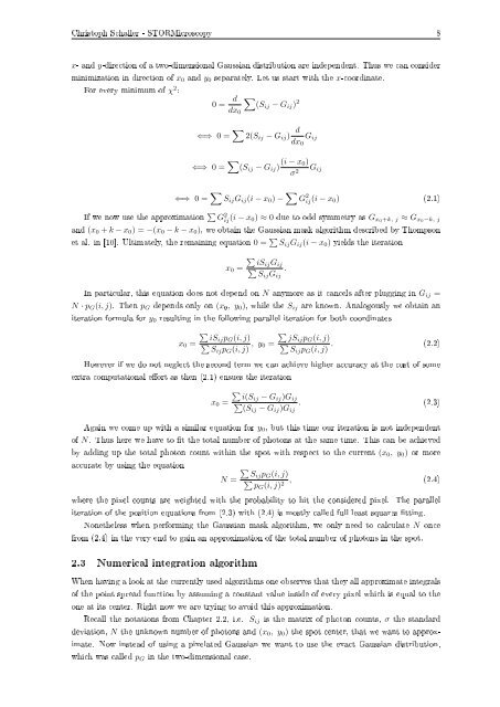
x- and y-direction of a two-dimensional Gaussian distribution are independent. Thus we can consider
minimization in direction of x 0 and y 0 separately. Let us start with the x-coordinate.
For every minimum of χ 2 :
0 = d
dx 0
∑
(Sij − G ij ) 2
⇐⇒ 0 = ∑ 2(S ij − G ij ) d
dx 0
G ij
⇐⇒ 0 = ∑ (S ij − G ij ) (i − x 0)
σ 2 G ij
⇐⇒ 0 = ∑ S ij G ij (i − x 0 ) − ∑ G 2 ij(i − x 0 ) (2.1)
If we now use the approximation ∑ G 2 ij (i − x 0) ≈ 0 due to odd symmetry as G x0+k, j ≈ G x0−k, j
and (x 0 + k − x 0 ) = −(x 0 − k − x 0 ), we obtain the Gaussian mask algorithm described by Thompson
et al. in [10]. Ultimately, the remaining equation 0 = ∑ S ij G ij (i − x 0 ) yields the iteration
x 0 =
∑
iSij G ij
∑
Sij G ij
.
In particular, this equation does not depend on N anymore as it cancels after plugging in G ij =
N · p G (i, j). Then p G depends only on (x 0 , y 0 ), while the S ij are known. Analogously we obtain an
iteration formula for y 0 resulting in the following parallel iteration for both coordinates
x 0 =
∑ ∑
iSij p G (i, j)
∑
Sij p G (i, j) , y jSij p G (i, j)
0 = ∑
Sij p G (i, j) . (2.2)
However if we do not neglect the second term we can achieve higher accuracy at the cost of some
extra computational eort as then (2.1) ensues the iteration
x 0 =
∑ i(Sij − G ij )G ij
∑
(Sij − G ij )G ij
. (2.3)
Again we come up with a similar equation for y 0 , but this time our iteration is not independent
of N. Thus here we have to t the total number of photons at the same time. This can be achieved
by adding up the total photon count within the spot with respect to the current (x 0 , y 0 ) or more
accurate by using the equation
∑
Sij p G (i, j)
N = ∑
pG (i, j) 2 , (2.4)
where the pixel counts are weighted with the probability to hit the considered pixel. The parallel
iteration of the position equations from (2.3) with (2.4) is mostly called full least squares tting.
Nonetheless when performing the Gaussian mask algorithm, we only need to calculate N once
from (2.4) in the very end to gain an approximation of the total number of photons in the spot.
2.3 Numerical integration algorithm
When having a look at the currently used algorithms one observes that they all approximate integrals
of the point spread function by assuming a constant value inside of every pixel which is equal to the
one at its center. Right now we are trying to avoid this approximation.
Recall the notations from Chapter 2.2, i.e. S ij is the matrix of photon counts, σ the standard
deviation, N the unknown number of photons and (x 0 , y 0 ) the spot center, that we want to approximate.
Now instead of using a pixelated Gaussian we want to use the exact Gaussian distribution,
which was called p G in the two-dimensional case.