Christoph Florian Schaller - FU Berlin, FB MI

Christoph Schaller - STORMicroscopy 14
3 Uncertainty and precision
Before the algorithms will be tested, we assess the inherent inaccuracies in the tting process.
3.1 Error estimation
In [10] Thompson et al. furthermore provided the single error estimation for the localization precision
of least squares tting. This is done by splitting up the problem into the two extreme cases of few or
many photons (compared to the background noise) being present.
We start with the so called photon shot noise-limited case, where we assume that no background
noise is present or it is negligible compared to the occuring photon numbers. As long as no pixelation
occurs the error can be estimated by the common statistical formula 〈(△x) 2 〉 = Var(x)
N
= σ2 . N
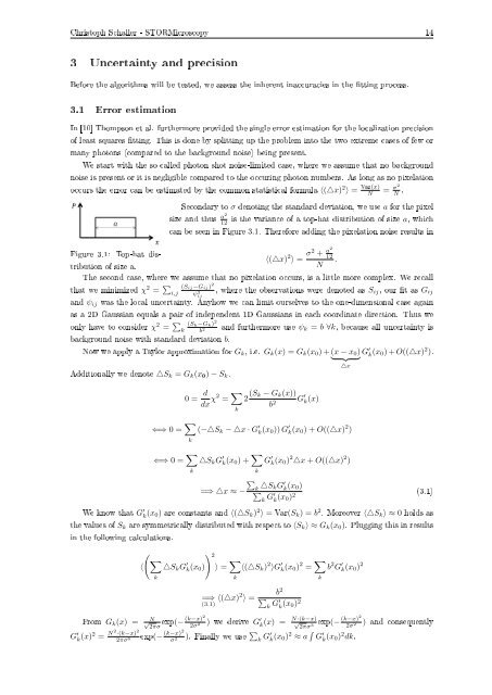
Secondary to σ denoting the standard deviation, we use a for the pixel
size and thus a2
12
is the variance of a top-hat distribution of size a, which
can be seen in Figure 3.1. Therefore adding the pixelation noise results in
Figure 3.1: Top-hat distribution
of size a.
N .
〈(△x) 2 〉 = σ2 + a2
12
The second case, where we assume that no pixelation occurs, is a little more complex. We recall
that we minimized χ 2 = ∑ (S ij−G ij) 2
i,j
, where the observations were denoted as S
ψij
2 ij , our t as G ij
and ψ ij was the local uncertainty. Anyhow we can limit ourselves to the one-dimensional case again
as a 2D Gaussian equals a pair of independent 1D Gaussians in each coordinate direction. Thus we
only have to consider χ 2 = ∑ (S k −G k ) 2
k b
and furthermore use ψ 2
k = b ∀k, because all uncertainty is
background noise with standard deviation b.
Now we apply a Taylor approximation for G k , i.e. G k (x) = G k (x 0 ) + (x − x 0 ) G ′ k
} {{ }
(x 0) + O((△x) 2 ).
△x
Additionally we denote △S k = G k (x 0 ) − S k .
0 = d
dx χ2 = ∑ k
2 (S k − G k (x))
b 2 G ′ k(x)
⇐⇒ 0 = ∑ k
(−△S k − △x · G ′ k(x 0 )) G ′ k(x 0 ) + O((△x) 2 )
⇐⇒ 0 = ∑ k
△S k G ′ k(x 0 ) + ∑ k
G ′ k(x 0 ) 2 △x + O((△x) 2 )
=⇒ △x ≈ −
∑
k △S kG ′ k (x 0)
∑k G′ k (x 0) 2 (3.1)
We know that G ′ k (x 0) are constants and 〈(△S k ) 2 〉 = Var(S k ) = b 2 . Moreover 〈△S k 〉 ≈ 0 holds as
the values of S k are symmetrically distributed with respect to 〈S k 〉 ≈ G k (x 0 ). Plugging this in results
in the following calculations.
( ∑
〈
k
) 2
△S k G ′ k(x 0 ) 〉 = ∑ k
〈(△S k ) 2 〉G ′ k(x 0 ) 2 = ∑ k
b 2 G ′ k(x 0 ) 2
From G k (x) =
G ′ k (x)2 = N 2·(k−x) 2
2πσ 6
√ N
2πσ
exp(− (k−x)2
2σ 2
exp(− (k−x)2
σ 2
=⇒
(3.1) 〈(△x)2 〉 =
b 2
∑
k G′ k (x 0) 2
) we derive G ′ N·(k−x)
k
(x) = √
2πσ 3
). Finally we use ∑ k G′ k (x 0) 2 ≈ a ´ G ′ k (x 0) 2 dk.
exp(− (k−x)2
2σ
) and consequently
2