Christoph Florian Schaller - FU Berlin, FB MI
Christoph Florian Schaller - FU Berlin, FB MI
Christoph Florian Schaller - FU Berlin, FB MI
Create successful ePaper yourself
Turn your PDF publications into a flip-book with our unique Google optimized e-Paper software.
<strong>Christoph</strong> <strong>Schaller</strong> - STORMicroscopy 10<br />
we can write<br />
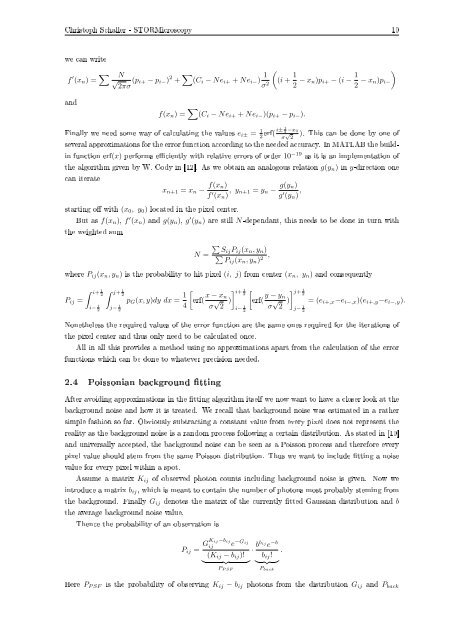
f ′ (x n ) = ∑<br />
N<br />
√ (p i+ − p i− ) 2 + ∑ (C i − Ne i+ + Ne i− ) 1 (<br />
2πσ σ 2 (i + 1 2 − x n)p i+ − (i − 1 )<br />
2 − x n)p i−<br />
and<br />
f(x n ) = ∑ (C i − Ne i+ + Ne i− )(p i+ − p i− ).<br />
Finally we need some way of calculating the values e i± = 1 2 erf( i± 1 2 −x0<br />
σ √ ). This can be done by one of<br />
2<br />
several approximations for the error function according to the needed accuracy. In MATLAB the buildin<br />
function erf(x) performs eciently with relative errors of order 10 −19 as it is an implementation of<br />
the algorithm given by W. Cody in [12]. As we obtain an analogous relation g(y n ) in y-direction one<br />
can iterate<br />
x n+1 = x n − f(x n)<br />
f ′ (x n ) , y n+1 = y n − g(y n)<br />
g ′ (y n ) ,<br />
starting o with (x 0 , y 0 ) located in the pixel center.<br />
But as f(x n ), f ′ (x n ) and g(y n ), g ′ (y n ) are still N-dependant, this needs to be done in turn with<br />
the weighted sum<br />
N =<br />
∑<br />
Sij P ij (x n , y n )<br />
∑<br />
Pij (x n , y n ) 2 ,<br />
where P ij (x n , y n ) is the probability to hit pixel (i, j) from center (x n , y n ) and consequently<br />
P ij =<br />
ˆ i+ 1<br />
2<br />
i− 1 2<br />
ˆ j+ 1<br />
2<br />
j− 1 2<br />
p G (x, y)dy dx = 1 4<br />
[<br />
erf( x − x ] i+ 1<br />
n<br />
σ √ 2 ) 2<br />
i− 1 2<br />
[<br />
erf( y − y ] j+ 1<br />
n<br />
σ √ 2 ) 2<br />
j− 1 2<br />
= (e i+,x −e i−,x )(e i+,y −e i−,y ).<br />
Nonetheless the required values of the error function are the same ones required for the iterations of<br />
the pixel center and thus only need to be calculated once.<br />
All in all this provides a method using no approximations apart from the calculation of the error<br />
functions which can be done to whatever precision needed.<br />
2.4 Poissonian background tting<br />
After avoiding approximations in the tting algorithm itself we now want to have a closer look at the<br />
background noise and how it is treated. We recall that background noise was estimated in a rather<br />
simple fashion so far. Obviously subtracting a constant value from every pixel does not represent the<br />
reality as the background noise is a random process following a certain distribution. As stated in [10]<br />
and universally accepted, the background noise can be seen as a Poisson process and therefore every<br />
pixel value should stem from the same Poisson distribution. Thus we want to include tting a noise<br />
value for every pixel within a spot.<br />
Assume a matrix K ij of observed photon counts including background noise is given. Now we<br />
introduce a matrix b ij , which is meant to contain the number of photons most probably steming from<br />
the background. Finally G ij denotes the matrix of the currently tted Gaussian distribution and b<br />
the average background noise value.<br />
Thence the probability of an observation is<br />
P ij = GKij−bij<br />
e −Gij<br />
(K ij − b ij )!<br />
} {{ }<br />
P P SF<br />
· bbij e −b<br />
.<br />
b ij !<br />
} {{ }<br />
P back<br />
Here P P SF is the probability of observing K ij − b ij photons from the distribution G ij and P back


