Christoph Florian Schaller - FU Berlin, FB MI

Christoph Schaller - STORMicroscopy 12
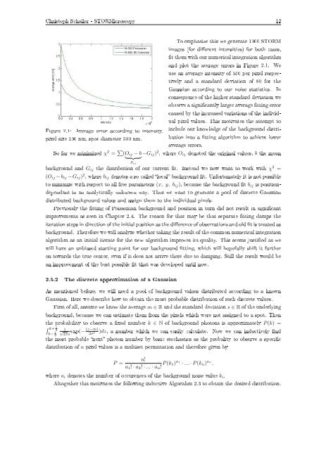
Figure 2.1: Average error according to intensity,
pixel size 100 nm, spot diameter 500 nm.
To emphasize this we generate 1000 STORM
images (for dierent intensities) for both cases,
t them with our numerical integration algorithm
and plot the average errors in Figure 2.1. We
use an average intensity of 550 per pixel respectively
and a standard deviation of 80 for the
Gaussian according to our noise statistics. In
consequence of the higher standard deviation we
observe a signicantly larger average tting error
caused by the increased variations of the individual
pixel values. This motivates the attempt to
include our knowledge of the background distribution
into a tting algorithm to achieve lower
average errors.
So far we minimized χ 2 = ∑ (O ij − b −G ij ) 2 , where O ij denoted the original values, b the mean
} {{ }
S ij
background and G ij the distribution of our current t. Instead we now want to work with χ 2 =
(O ij − b ij − G ij ) 2 , where b ij denotes a so called local background t. Unfortunately it is not possible
to minimize with respect to all free parameters (x, y, b ij ), because the background t b ij is positiondependant
in an analytically unknown way. Thus we want to generate a pool of discrete Gaussian
distributed background values and assign them to the individual pixels.
Previously the tting of Poissonian background and position in turn did not result in signicant
improvements as seen in Chapter 2.4. The reason for that may be that separate tting damps the
iteration steps in direction of the initial position as the dierence of observations and old t is treated as
background. Therefore we will analyze whether taking the result of the common numerical integration
algorithm as an initial iterate for the new algorithm improves its quality. This seems justied as we
will have an unbiased starting point for our background tting, which will hopefully shift it further
on towards the true center, even if it does not arrive there due to damping. Still the result would be
an improvement of the best possible t that was developed until now.
2.5.2 The discrete approximation of a Gaussian
As mentioned before, we will need a pool of background values distributed according to a known
Gaussian. Here we describe how to obtain the most probable distribution of such discrete values.
First of all, assume we know the average m ∈ R and the standard deviation s ∈ R of the underlying
background, because we can estimate them from the pixels which were not assigned to a spot. Then
the probability to observe a xed number k ∈ N of background photons is approximately P (k) =
´ k+ 1
2
k− 1 2
√ 1
2πs
exp(− (z−m)
2s
)dz, a number which we can easily calculate. Now we can inductively nd
2
the most probable next photon number by basic stochastics as the probality to observe a specic
distribution of n pixel values is a multiset permutation and therefore given by
P =
n!
a 1 ! · a 2 ! · ... · a n ! P (k 1) a1 · ... · P (k n ) an ,
where a i denotes the number of occurences of the background noise value k i .
Altogether this motivates the following inductive Algorithm 2.3 to obtain the desired distribution.