Christoph Florian Schaller - FU Berlin, FB MI

Christoph Schaller - STORMicroscopy 32
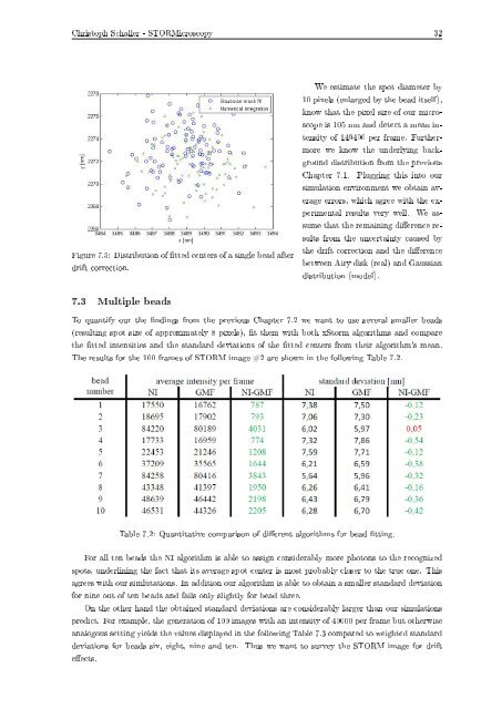
Figure 7.5: Distribution of tted centers of a single bead after
drift correction.
We estimate the spot diameter by
10 pixels (enlarged by the bead itself),
know that the pixel size of our microscope
is 105 nm and detect a mean intensity
of 149400 per frame. Furthermore
we know the underlying background
distribution from the previous
Chapter 7.1. Plugging this into our
simulation environment we obtain average
errors, which agree with the experimental
results very well. We assume
that the remaining dierence results
from the uncertainty caused by
the drift correction and the dierence
between Airy disk (real) and Gaussian
distribution (model).
7.3 Multiple beads
To quantify our the ndings from the previous Chapter 7.2 we want to use several smaller beads
(resulting spot size of approximately 8 pixels), t them with both xStorm algorithms and compare
the tted intensities and the standard deviations of the tted centers from their algorithm's mean.
The results for the 100 frames of STORM image #2 are shown in the following Table 7.2.
Table 7.2: Quantitative comparison of dierent algorithms for bead tting.
For all ten beads the NI algorithm is able to assign considerably more photons to the recognized
spots, underlining the fact that its average spot center is most probably closer to the true one. This
agrees with our simlutations. In addition our algorithm is able to obtain a smaller standard deviation
for nine out of ten beads and fails only slightly for bead three.
On the other hand the obtained standard deviations are considerably larger than our simulations
predict. For example, the generation of 100 images with an intensity of 40000 per frame but otherwise
analogous setting yields the values displayed in the following Table 7.3 compared to weighted standard
deviations for beads six, eight, nine and ten. Thus we want to survey the STORM image for drift
eects.