Christoph Florian Schaller - FU Berlin, FB MI

Christoph Schaller - STORMicroscopy 30
7 Experimental observations
In the end we analyze the experimental data. Some basic results are displayed here.
7.1 Noise statistics
As a start we want to have a look at the background noise. To do so we consider all pixels within a
40 × 41 grid of a common STORM image (#1, 100 frames), that were part of no tted spot. Then
we collect the occuring intensities, which are proportional to the photon numbers, into several bins.
Finally normalizing the data results in the attached Figure 7.1.
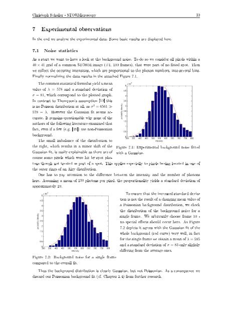
Figure 7.1: Experimental background noise tted
with a Gaussian.
The common statistical formulas yield a mean
value of λ = 578 and a standard deviation of
σ = 81, which correspond to the plotted graph.
In contrast to Thompson's assumption [10] this
is no Poisson distribution at all, as σ 2 = 6561 ≫
578 = λ. However the Gaussian t seems accurate.
It remains questionable why none of the
authors of the following literature examined that
fact, even if a few (e.g. [19]) use non-Poissonian
background.
The small imbalance of the distribution to
the right, which results in a minor shift of the
Gaussian t, is easily explainable as there are of
course some pixels which were hit by spot photons
though not treated as part of a spot. This applies especially to pixels beeing located in one of
the outer rings of an Airy distribution.
One has to pay attention to the dierence between the intensity and the number of photons
here. Assuming a mean of 130 photons per pixel, the proportionality yields a standard deviation of
approximately 20.
Figure 7.2: Background noise for a single frame
compared to the overall t.
To ensure that the increased standard deviation
is not the result of a changing mean value of
a Poissonian background distribution, we check
the distribution of the background noise for a
single frame. We arbitrarily choose frame 50 -
no special eects should occur here. As Figure
7.2 depicts it agrees with the Gaussian t of the
whole background (red curve) very well, in fact
for the single frame we obtain a mean of λ = 585
and a standard deviation of σ = 83 only slightly
diering from the average ones.
Thus the background distribution is clearly Gaussian, but not Poissonian. As a consequence we
discard our Poissonian background t (cf. Chapter 2.4) from further research.