Christoph Florian Schaller - FU Berlin, FB MI

Christoph Schaller - STORMicroscopy 16
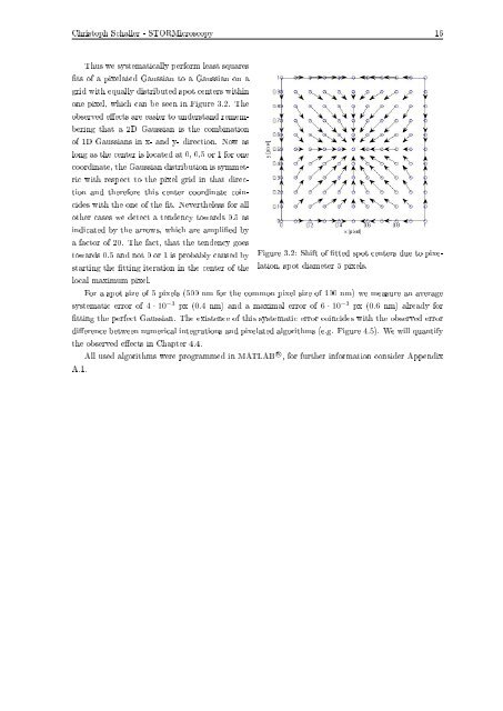
Thus we systematically perform least squares
ts of a pixelated Gaussian to a Gaussian on a
grid with equally distributed spot centers within
one pixel, which can be seen in Figure 3.2. The
observed eects are easier to understand remembering
that a 2D Gaussian is the combination
of 1D Gaussians in x- and y- direction. Now as
long as the center is located at 0, 0.5 or 1 for one
coordinate, the Gaussian distribution is symmetric
with respect to the pixel grid in that direction
and therefore this center coordinate coincides
with the one of the t. Nevertheless for all
other cases we detect a tendency towards 0.5 as
indicated by the arrows, which are amplied by
a factor of 20. The fact, that the tendency goes
towards 0.5 and not 0 or 1 is probably caused by
starting the tting iteration in the center of the
local maximum pixel.
Figure 3.2: Shift of tted spot centers due to pixelation,
spot diameter 5 pixels.
For a spot size of 5 pixels (500 nm for the common pixel size of 100 nm) we measure an average
systematic error of 4 · 10 −3 px (0.4 nm) and a maximal error of 6 · 10 −3 px (0.6 nm) already for
tting the perfect Gaussian. The existence of this systematic error coincides with the observed error
dierence between numerical integrations and pixelated algorithms (e.g. Figure 4.5). We will quantify
the observed eects in Chapter 4.4.
All used algorithms were programmed in MATLAB R○ , for further information consider Appendix
A.1.