1.1 The Radiation Laws and the Birth of Quantum Mechanics

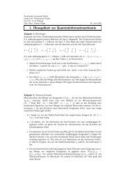
QUANTUM MECHANICS I (Dr. T. Brandes): Example/Solution Sheets 16
2.10.5 ** A more general definition of the transfer matrix M (> 30 min)
We consider a one–dimensional potential of the form
⎧
⎧
⎨ 0,
⎨ ae ikx + be −ikx , −∞ < x ≤ x 1
V (x) = v(x), ψ(x) = φ(x), x 1 < x ≤ x 2
⎩
⎩
0
ce ikx + de −ikx , x 2 < x < ∞
(2.84)
Here, v(x) is an arbitrary real potential. The central part φ(x) of the wave function ψ(x)
therefore in general is very difficult to calculate. We can, however, relate the coefficients a, b
(left side) with the coefficients c, d (right side): if some fixed values for c and d are chosen,
this determines the solution ψ(x) everywhere on the x–axis and therefore in particular a and
b. We write this relation as
(
a
b
) ( ) (
M11 M
=
12 c
M 22 d
M 21
)
. (2.85)
a) With ψ(x) also the conjugate complex ψ ∗ (x) must be a solution of the stationary Schrödinger
equation Ĥψ(x) = Eψ(x). Why
b) Take the conjugate complex ψ ∗ (x) in (2.84) and show that this leads to the exchange a ↔ b ∗
and c ↔ d ∗ in (2.85).
c) Take the conjugate complex of the whole equation (2.85) and compare with the equation
you obtain from part b). Show that
d) Consider the current density and show that
M ∗ 11 = M 22 , M ∗ 12 = M 21 . (2.86)
|a| 2 − |b| 2 = |c| 2 − |d| 2 . (2.87)
Write this equation as a scalar product of vectors in the form
( ) ( ) ( ) (
1 0 a 1 0 c
(a ∗ b ∗ )
= (c ∗ d ∗ )
0 −1 b
0 −1 d
Use the matrix M to derive from this
)
. (2.88)
det(M) = 1. (2.89)
3.11 Axioms of Quantum Mechanics and the Hilbert Space
3.11.1 Definition (2min)
What is a Hilbert space
Def.: A Hilbert space is a complete unitary space.
3.11.2 Orthonormality (5 min)
Consider the Hilbert space H of wave functions ψ(x) of the infinite potential well on the
interval [0, L] with ψ(0) = ψ(L) = 0. Show that the basis vectors
√
2
( nπx
)
ψ n (x) =
L sin L
form an orthonormal system.