1.1 The Radiation Laws and the Birth of Quantum Mechanics

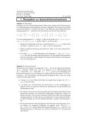
QUANTUM MECHANICS I (Dr. T. Brandes): Example/Solution Sheets 18
b) Show that in the case of vectors x, y ∈ R d , this reduces to the standard formula for the
scalar product in R d ,
d∑
〈x|y〉 = x ∗ i y i .
c) Use Eq.(3.91) and Eq.(3.90) to prove
i=1
π 6 ∞
960 = ∑ 1
(2k + 1) 6
3.12 Operators and Measurements in Quantum Mechanics
3.12.1 Definitions (2 min)
Show that the momentum operator ˆp = −i∇ is a linear operator.
Apply −i∇ to a linear combination of two wave functions.
3.12.2 Adjoint operator (10 min)
k=0
Consider the complex two–dimensional Hilbert space with basis vectors (1, 0) and (0, 1). Use
the definition of the adjoint operator to prove the following for the adjoint A † of the operator
A: If A is given as a complex two–by– two matrix,
( ) ( )
a b
a
A = A † ∗
c
=
∗
c d
b ∗ d ∗ .
Def.: The adjoint operator A † of a linear operator A acting on a Hilbert space H is defined by
We calculate the scalar products with the basis vectors e 1 , e 2 :
〈ψ|Aφ〉 = 〈A † ψ|φ〉, ∀φ, ψ ∈ H. (3.92)
A 11 = (e 1 , Ae 1 ) = a = (A † e 1 , e 1 ) = (A † 11 e 1, e 1 ) =
(
A † 11) ∗
. (3.93)
By this we have the element A † 11 of the adjoint matrix of A. Here, we used the fact that a scalar
c in the first argument of the scalar product appears as its conjugate complex when pulled out,
(cψ, φ) = c ∗ (ψ, φ). In completely the same manner we prove it for the other matrix elements.
3.12.3 Observables (5 min)
Which of the following matrices could describe physical observables in a Hilbert space of two
states
( ) ( ) ( ) ( )
1 1
−1 0
−100 i + 1
0 −i
A = , B =
, C =
, D =
.
0 2
0 0
i + 1 2
i 0
Physical observabes are represented hermitian operators. Def.: A linear operator A on the Hilbert
space H is called hermitian, if the following relation holds:
〈Aψ|φ〉 = 〈ψ|Aφ〉, ∀φ, ψ ∈ H. (3.94)
Therefore, only B and D describe physical observables. For example, B could describe a two level
atom in the basis of its two eigenstates with energy −1 and 0 (in some energy unit). D is the Pauli