Connes-Chern Character for Manifolds with Boundary and ETA ...

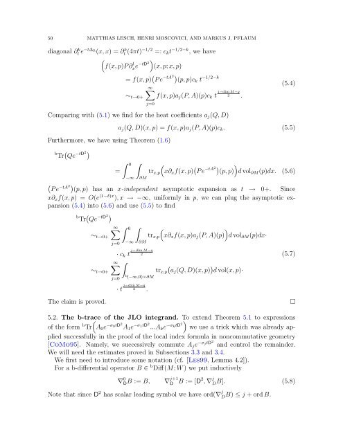
50 MATTHIAS LESCH, HENRI MOSCOVICI, AND MARKUS J. PFLAUM
diagonal ∂ k t e −t∆ R (x, x) = ∂
k
t (4πt) −1/2 =: c k t −1/2−k , we have
(
f(x, p)P ∂ l xe −tD2) (x, p; x, p)
= f(x, p) ( P e −tA2 )
(p, p)ck t −1/2−k
∼ t→0+
∞
∑
j=0
j−dim M−q
f(x, p)a j (P, A)(p)c k t 2 .
Comparing with (5.1) we find for the heat coefficients a j (Q, D)
Furthermore, we have using Theorem (1.6)
b Tr ( Qe −tD2 )
=
(5.4)
a j (Q, D)(x, p) = f(x, p)a j (P, A)(p)c k . (5.5)
∫ 0
−∞
∫
∂M
tr x,p
(
x∂ x f(x, p) ( P e −tA2 )
(p, p)
)d vol ∂M (p)dx. (5.6)
(
P e
−tA 2 )
(p, p) has an x-independent asymptotic expansion as t → 0+. Since
x∂ x f(x, p) = O(e (1−δ)x ), x → −∞, uniformly in p, we can plug the asymptotic expansion
(5.4) into (5.6) and use (5.5) to find
b Tr ( Qe −tD2 )
∼ t→0+
∼ t→0+
The claim is proved.
∑ ∞ ∫ 0
j=0
−∞
∫
∂M
j−dim M−q
· c k t 2
∫
∞
∑
j=0
b (−∞,0)×∂M
j−dim M−q
· t 2 .
)
tr x,p
(x∂ x f(x, p)a j (P, A)(p) d vol ∂M (p)dx·
tr x,p
(
aj (Q, D)(x, p) ) d vol(x, p)·
(5.7)
5.2. The b-trace of the JLO integrand. To ) extend Theorem 5.1 to expressions
of the form b Tr
(A 0 e −σ 0tD 2 A 1 e −σ 1tD 2 ...A k e −σ ktD 2 we use a trick which was already applied
successfully in the proof of the local index formula in noncommutative geometry
[CoMo95]. Namely, we successively commute A j e −σ jtD 2
and control the remainder.
We will need the estimates proved in Subsections 3.3 and 3.4.
We first need to introduce some notation (cf. [Les99, Lemma 4.2]).
For a b-differential operator B ∈ b Diff(M; W ) we put inductively
∇ 0 DB := B, ∇ j+1
D B := [D2 , ∇ j DB]. (5.8)
Note that since D 2 has scalar leading symbol we have ord(∇ j DB) ≤ j + ord B.
□