Connes-Chern Character for Manifolds with Boundary and ETA ...

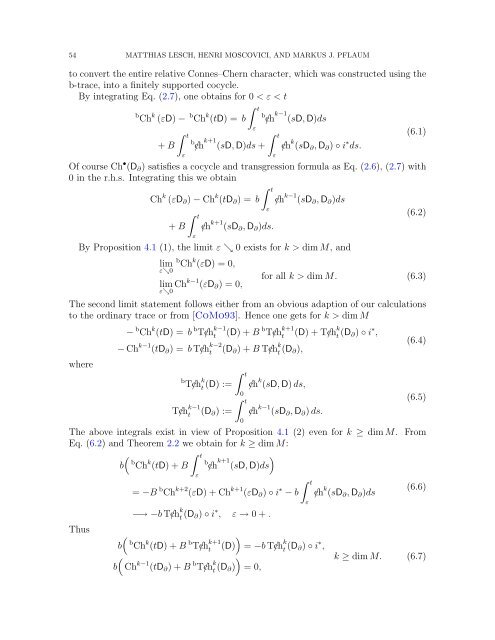
54 MATTHIAS LESCH, HENRI MOSCOVICI, AND MARKUS J. PFLAUM
to convert the entire relative Connes–Chern character, which was constructed using the
b-trace, into a finitely supported cocycle.
By integrating Eq. (2.7), one obtains for 0 < ε < t
b Ch k (εD) − b Ch k (tD) = b
+ B
∫ t
ε
∫ t
b /ch k+1 (sD, D)ds +
ε
b /ch k−1 (sD, D)ds
∫ t
ε
/ch k (sD ∂ , D ∂ ) ◦ i ∗ ds.
(6.1)
Of course Ch • (D ∂ ) satisfies a cocycle and transgression formula as Eq. (2.6), (2.7) with
0 in the r.h.s. Integrating this we obtain
Ch k (εD ∂ ) − Ch k (tD ∂ ) = b
+ B
∫ t
ε
∫ t
/ch k+1 (sD ∂ , D ∂ )ds.
ε
/ch k−1 (sD ∂ , D ∂ )ds
By Proposition 4.1 (1), the limit ε ↘ 0 exists for k > dim M, and
lim
b Ch k (εD) = 0,
ε↘0
lim
ε↘0 Chk−1 (εD ∂ ) = 0,
(6.2)
for all k > dim M. (6.3)
The second limit statement follows either from an obvious adaption of our calculations
to the ordinary trace or from [CoMo93]. Hence one gets for k > dim M
where
− b Ch k (tD) = b b T/ch k−1
t
(D) + B b T/ch k+1
t
(D) + T/ch k t (D ∂) ◦ i ∗ ,
− Ch k−1 (tD ∂ ) = b T/ch k−2
t
(D ∂ ) + B T/ch k t (D ∂),
∫ t
b T/ch k t (D) := /ch k (sD, D) ds,
T/ch k−1
t
(D ∂ ) :=
0
∫ t
0
/ch k−1 (sD ∂ , D ∂ ) ds.
(6.4)
(6.5)
The above integrals exist in view of Proposition 4.1 (2) even for k ≥ dim M. From
Eq. (6.2) and Theorem 2.2 we obtain for k ≥ dim M:
(
∫ t
)
b
b Ch k (tD) + B
b /ch k+1 (sD, D)ds
Thus
b
(
b
(
ε
= −B b Ch k+2 (εD) + Ch k+1 (εD ∂ ) ◦ i ∗ − b
−→ −b T/ch k t (D ∂) ◦ i ∗ , ε → 0 + .
b Ch k (tD) + B b T/ch k+1
t
)
(D)
)
Ch k−1 (tD ∂ ) + B b T/ch k t (D ∂)
∫ t
= −b T/ch k t (D ∂) ◦ i ∗ ,
= 0,
ε
/ch k (sD ∂ , D ∂ )ds
(6.6)
k ≥ dim M. (6.7)