Sequence Comparison.pdf

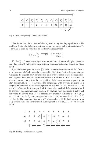
26 2 Basic Algorithmic Techniques
Fig. 2.7 Computing F 10 by a tabular computation.
Now let us describe a more efficient dynamic-programming algorithm for this
problem. Define S[i] to be the maximum sum of segments ending at position i of A.
The value S[i] can be computed by the following recurrence:
{
ai + max{S[i − 1],0} if i > 1,
S[i]=
a 1 if i = 1.
If S[i − 1] < 0, concatenating a i with its previous elements will give a smaller
sum than a i itself. In this case, the maximum-sum segment ending at position i is a i
itself.
By a tabular computation, each S[i] can be computed in constant time for i from 1
to n, therefore all S values can be computed in O(n) time. During the computation,
we record the largest S entry computed so far in order to report where the maximumsum
segment ends. We also record the traceback information for each position i so
that we can trace back from the end position of the maximum-sum segment to its
start position. If S[i − 1] > 0, we need to concatenate with previous elements for a
larger sum, therefore the traceback symbol for position i is “←.” Otherwise, “↑” is
recorded. Once we have computed all S values, the traceback information is used
to construct the maximum-sum segment by starting from the largest S entry and
following the arrows until a “↑” is reached. For example, in Figure 2.8, A = 〈3, 2,
-6,5,2,-3,6,-4,2〉. By computing from i = 1toi = n, wehaveS = 〈3, 5, -1, 5, 7,
4, 10,6, 8〉. The maximum S entry is S[7] whose value is 10. By backtracking from
S[7], we conclude that the maximum-sum segment of A is 〈5, 2, -3, 6〉, whose sum
is 10.
Fig. 2.8 Finding a maximum-sum segment.